A Calibrated Screening Dataset of Magnetocrystalline Anisotropy for Rare-Earth-Free Magnet Discovery

Magnet-Anisotropy-Screening

Will Bryan, Matt Moderwell · ghost-projects · July 2026

Abstract

Magnetocrystalline anisotropy is the property that separates a permanent magnet from a merely magnetic material, and it is the scarcest label in public materials databases: the large repositories record magnetic moments and orderings but not the anisotropy constant $K_1$, because computing it requires relativistic density functional theory that costs orders of magnitude more than a standard relaxation. We present a screening-scale dataset of 3,573 uniaxial inorganic crystals, 2,242 of them carrying a computed anisotropy label ($K_1$, saturation magnetization $M_s$, the dimensionless magnetic hardness $\kappa = \sqrt{K_1/\mu_0 M_s^2}$, and the easy-axis direction), alongside Curie temperature, energy above the convex hull, and, for compounds that pass every screening gate, a micromagnetic estimate of the achievable energy product. Relaxed atomic structures accompany 88% of the labeled entries. The dataset’s distinguishing feature is its error model. A stratified subset of 287 compounds was recomputed at tightened density-functional settings, which separates the label error into a small systematic bias (a per-$\kappa$-band median correction of 0–4%, applied to the shipped values) and a substantial per-label scatter (interquartile range of ±16% in the magnet-relevant bands, with only 48% of labels within ±10% of their high-accuracy value). An eleven-compound benchmark against literature values confirms the pipeline recovers the correct hardness ordering and easy axis for well-defined hard magnets at density-functional-theory magnitudes, which for the hardest magnets exceed room-temperature experiment by the well-documented factor of 1.5–2. The dataset is released as a screening and machine-learning resource with its noise floor stated: models trained on it should not be expected to regress $\kappa$ better than roughly ±15–20%.

1 Background and summary

The strongest permanent magnets in production, the Nd–Fe–B family [1], depend on rare-earth elements whose supply is concentrated and volatile, and the search for rare-earth-free replacements has run for four decades without displacing them. What makes the search hard is a conjunction: a viable permanent magnet needs a large saturation magnetization, a Curie temperature comfortably above its operating range, thermodynamic stability, and, as the discriminating requirement, enough magnetocrystalline anisotropy to resist demagnetization. The conventional threshold is a magnetic hardness $\kappa = \sqrt{K_1/\mu_0 M_s^2}$ greater than one [2], which permits a magnet of any shape without self-demagnetizing. Iron-rich compounds deliver magnetization cheaply; anisotropy is the property that is scarce.

Anisotropy data is scarce for a practical reason. The property arises from spin–orbit coupling, so computing $K_1$ requires fully-relativistic density functional theory with dense Brillouin-zone sampling: typically tens of minutes to hours per compound even at screening settings, against seconds for the machine-learned relaxations that populate modern databases. The Materials Project [4] and similar repositories consequently record magnetic moments and ground-state orderings but not $K_1$; MAGNDATA [5] catalogs roughly two thousand experimentally determined magnetic structures, again without anisotropy constants. The closest comparable resource, Novamag [6], computed ab initio properties for a magnet-focused set of similar scale, but without a quantified account of how converged its labels are. A researcher training a structure-to-anisotropy model today has no public bulk dataset that states its own noise floor.

This report describes such a dataset. It contains 3,573 screened uniaxial crystals, 2,242 anisotropy labels computed with a single consistent method (Green’s-function magnetic-interaction extraction over fully-relativistic density functional theory), relaxed atomic structures for 88% of the labeled entries, and a calibration tier of 287 compounds recomputed at tightened settings, from which we derive both the systematic bias of the production labels, which is small and corrected in the shipped values, and their per-label scatter, which dominates the error budget and is quantified. The dataset spans soft and hard, stable and metastable, easy-axis and easy-plane compounds in roughly even proportion, because negative examples carry as much training signal as positives for a screening model.

Three design choices frame the dataset’s scope. First, only uniaxial crystal systems (tetragonal, hexagonal, trigonal) are included, since only these support the single easy axis a permanent magnet requires. Second, rare-earth elements are absent by construction: the pseudopotential set behind the anisotropy calculation contains no lanthanides, which matches the dataset’s purpose of rare-earth-free discovery. Precious-metal compounds (Pt, Pd, Ir, Rh) are included as positive examples of high anisotropy and are identifiable by composition. Third, every label was computed through the same relaxation and the same settings, so the dataset is internally consistent: comparisons across entries reflect the materials, not method differences.

Table 1 places the release among existing resources with magnetic labels.

Table 1. Public resources with magnetic labels. Anisotropy constants are the gap this dataset addresses.

resource	scale	$K_1$ labels	notes
Materials Project [4]	~150k bulk	none	moments and orderings, no anisotropy
AFLOW [17]	millions	none	—
MAGNDATA [5]	~2k	none	experimental magnetic structures
Novamag [6]	~2k magnet-focused	partial	closest comparable; no convergence/error model
C2DB [7]	~4k	yes	two-dimensional materials, different domain
this work	3,573 uniaxial bulk	2,242 (2,044 reliable)	per-label error model, relaxed structures, negatives

Two features distinguish this dataset from the table’s nearest neighbor. Novamag reports ab initio values without a convergence account, so a user cannot separate model error from label error; Section 5 quantifies that difference here. And this dataset keeps its rejects: 2,735 records failed a gate, and those that failed after the anisotropy stage still carry valid labels, the negative examples a model needs to learn the boundary of the viable region rather than only its interior.

The report follows the conventions of a data descriptor [18]. Section 2 builds intuition for the labels in pictures, Section 3 describes how the dataset was constructed, Section 4 presents the data record and its statistics, Section 5 the technical validation against refined settings and literature, and Section 6 usage notes.

2 What the labels measure

Four numbers do most of the work in this dataset (the saturation magnetization $M_s$, the anisotropy constant $K_1$, the hardness $\kappa$, and the energy product $(BH)_{max}$), and the relationships between them decide whether a compound is a permanent magnet. This section builds the intuition for each in pictures; readers who work with magnets can skip to Section 3.

2.1 Anisotropy energy and the easy axis

Below its Curie temperature a ferromagnet’s moments align, giving a net magnetization of magnitude $M_s$ per unit volume. Alignment alone says nothing about direction: exchange interactions, which cause the ordering, are isotropic. Direction enters through spin–orbit coupling, which ties the moments to the crystal lattice and makes the energy depend on the angle $\theta$ between the magnetization and the crystal’s unique axis. To leading order in a uniaxial crystal [3],

$$E(\theta) \;=\; K_1 \sin^2\theta$$

When $K_1 > 0$ the energy has two minima, along $+c$ and $-c$: an easy axis. The barrier between them is $K_1$ per unit volume, and that barrier is what lets the material hold a magnetization direction (store a pole) against time, temperature, and stray fields. When the minimum lies at $\theta = 90°$ instead, every direction in the basal plane is equally good: an easy plane, a continuous ring of minima with no barrier between them, around which the magnetization rotates at negligible cost. An easy-plane material cannot hold a pole no matter how large its anisotropy energy is. The dataset therefore reports the easy-axis label (001 versus in-plane) as a first-class output: it decides magnet viability before any question of magnitude.

Figure 1. Magnetocrystalline anisotropy is an energy landscape over the magnetization direction. Left: in an easy-axis material the two minima along ±c are separated by a barrier of $K_1$ per unit volume, the physical quantity every anisotropy label in this dataset measures. Right: the L1₀ unit cell of FePt, in which Pt (gray) and Fe (orange) occupy alternating layers along c, and that layering is what singles out the axis. The same uniaxial cell admits two outcomes: minima along ±c (easy axis, M holds a direction) or a degenerate ring of minima in the basal plane (easy plane, M rotates freely and no direction is retained). The axis-versus-plane label therefore matters before any magnitude does.

2.2 Hardness: anisotropy versus the magnet’s own field

The poles a magnetized body develops generate a demagnetizing field inside the body that points against the magnetization, and the energy scale of that self-field is $\mu_0 M_s^2$, so the drive to demagnetize grows with the square of the magnetization. What resists is the anisotropy barrier $K_1$. The dimensionless hardness

$$\kappa \;=\; \sqrt{\frac{K_1}{\mu_0 M_s^2}}$$

compares the two scales, and its practical meaning is geometric: when $\kappa > 1$ the anisotropy wins in the worst case, so the material can be made into a magnet of any shape; below that, a compact body demagnetizes itself, and only elongated geometries survive [2]. This is why raw magnetization is not enough. Iron has one of the largest $M_s$ values known and is magnetically useless as a permanent magnet: its anisotropy is two orders of magnitude too small for its own field.

Figure 2. Hardness is a ratio of two energy scales. Iron carries an enormous magnetization (tall gray bar, µ₀Ms² ≈ 3.7 MJ/m³) but almost no anisotropy to defend it (K₁ ≈ 0.05), so it demagnetizes itself: κ ≈ 0.1. Nd₂Fe₁₄B and L1₀ FePt hold less magnetization but defend it with anisotropy several times the self-field scale. The dataset's κ label encodes this contest for every entry, and the κ = 1 line in Figure 6 is the boundary where the orange bar starts winning.

2.3 From intrinsic numbers to a working magnet

A permanent magnet is used to deliver flux outside its own volume, and that performance is read off the hysteresis loop: the magnet’s flux density $B$ as the opposing field $H$ it must work against increases. Three figures of merit live on the loop, and each traces back to an intrinsic label in this dataset. The remanence $B_r$, the flux density retained at zero applied field, is capped by $\mu_0 M_s$. The coercivity $H_c$, the reverse field the magnet withstands before its magnetization flips, is capped by the anisotropy field $2K_1/\mu_0 M_s$, although real magnets reach only a fraction of that cap, because reversal nucleates early at grain boundaries and defects [3]. The energy product $(BH)_{max}$, the standard single figure of merit, is the largest $B \times H$ rectangle that fits under the second-quadrant curve, with a theoretical ceiling of $\mu_0 M_s^2/4$ for a square loop.

The gap between the intrinsic ceilings and what a manufactured magnet delivers is decided by microstructure: grain size, crystallographic texture, grain-boundary chemistry, soft-phase inclusions. That is why the pipeline’s final stage (Section 3.1) sweeps 2,000 sampled microstructures per gate-passing compound: the peak $(BH)_{max}$ estimates the ceiling, and the robustness score estimates how forgiving the compound is of imperfect processing. Temperature closes the loop’s story: every one of these properties decays toward zero at the Curie temperature, which is why a $T_c$ comfortably above the operating range is a gate in its own right.

Figure 3. How the intrinsic labels become a magnet's spec sheet. The hysteresis loop's second quadrant (shaded region) is where a permanent magnet operates, working against its own demagnetizing field. $M_s$ caps the remanence, $K_1$ caps the coercivity, and the largest rectangle under the curve is the energy product, with ceiling $\mu_0 M_s^2/4$. Microstructure decides how much of each ceiling survives manufacturing, which is what the pipeline's final sweep stage estimates.

3 Methods

3.1 Screening cascade

Every record passed through the same staged pipeline, ordered so the expensive anisotropy calculation is only paid for structures that are physical, uniaxial, and magnetic. Property calculations ran as hosted routes on the Ouro platform [16]; orchestration ran on Modal.

Figure 4. The screening funnel. Records that fail a gate are retained: any compound that reached the anisotropy stage keeps its label, so the 2,242 labeled entries include easy-plane, soft, and metastable negatives alongside the 641 that clear every gate.

The stages, with their exact settings:

Relaxation. Orb-v3 machine-learned interatomic potential (orb-v3-conservative-inf-mpa) [8], force convergence 0.05 eV/Å, at most 200 steps. Structures whose relaxed nearest-neighbor distance fell below 1.5 Å were rejected as unphysical. The relaxed structure, not the input, feeds every later stage.
Symmetry. Only tetragonal, hexagonal, and trigonal cells proceed. Space group and crystal system are recorded from the relaxed cell.
Stability. Energy above the convex hull, referenced against the Materials Project hull, recorded in meV/atom.
Intrinsic magnetism. Curie temperature and magnetization density from dedicated property models [16]; the Curie estimate should be treated as method-level (such estimates typically run high).
Anisotropy. The expensive stage, described in Section 3.2. Outputs $K_1$, $M_s$, $\kappa$, and the easy-axis direction.
Microstructure sweep (gate-passing compounds only). A micromagnetic proxy model sweeps seven microstructure parameters (degree of chemical order, texture spread, grain size, grain-boundary exchange and magnetization, soft-phase fraction, dead-layer thickness) over 2,000 Latin-hypercube samples, reporting the peak energy product $(BH)_{max}$, peak remanence, and a robustness score: the share of sampled microstructures that clear coercivity ≥ 600 kA/m, remanence ≥ 0.8 T, and $(BH)_{max}$ ≥ 100 kJ/m³, weighted by their margin above those thresholds.

Figure 5. The microstructure sweep of stage 6. Left: the object the sweep parameterizes, a textured polycrystal in which each grain's shade encodes its misalignment from the pressing axis, grain boundaries carry reduced exchange and magnetization, and the gray pockets at the triple junctions are soft phase. Right: real sweep output for HfGaFe₄, the 2,000 Latin-hypercube samples aggregated onto the two most sensitive axes. The share of samples clearing all three thresholds concentrates at high chemical order and low grain-boundary exchange; that concentration is the acceptable window the dataset reports for each gate-passing compound.

Two gate configurations were used. The discovery configuration enforces magnet-viability floors (Curie temperature ≥ 400 K, $M_s$ ≥ 0.5 MA/m, hull distance ≤ 200 meV/atom, $\kappa > 1$, easy axis along the crystallographic c-axis). The dataset-building configuration relaxes those floors (Curie ≥ 0 K, $M_s$ ≥ 0.1 MA/m, hull distance ≤ 500 meV/atom) so that the anisotropy label is captured for any uniaxial magnetic structure, including ones that make poor magnets. Most of the dataset was built in the second configuration, which is why its label distribution covers soft and hard compounds alike. The anisotropy stage dominates the cost: a production calculation takes 8 to 15 minutes per compound and the high-accuracy recomputations up to several hours, for roughly 2,900 anisotropy calculations in total over the eight-day screening period.

3.2 The anisotropy calculation

Each anisotropy label comes from TB2J [10] magnetic-interaction extraction over ABACUS [9] density-functional-theory calculations with the PseudoDojo fully-relativistic norm-conserving pseudopotential set (Dojo-NC-FR) [11]. Production settings are a k-point spacing of 0.16 Å⁻¹ and a plane-wave cutoff of 65 Ry; the calibration tier of Section 5 tightens these to 0.10 Å⁻¹ and 80 Ry. The calculation assumes ferromagnetic alignment of the moments (a limitation quantified by a dedicated flag, Section 6) and reports the anisotropy energy resolved along the crystal axes, from which the easy axis and $K_1$ follow. In uniaxial cells the two in-plane directions are degenerate, so the meaningful easy-axis distinction is axis (001) versus plane (100/010), and that is the distinction the error analysis of Section 5 uses.

The pseudopotential set contains no lanthanides or actinides, so rare-earth compounds cannot be computed, a hard constraint that defines the dataset’s scope. Everything else, including the 5d precious metals, is computable, and 160 of the reliable labels contain a precious metal; these serve as high-anisotropy positive examples (the L1₀ family among them) and are trivially excluded by composition when a strictly precious-free view is wanted.

3.3 Sources

Table 2. Provenance of the 3,573 records. Each record’s source column carries its tag.

source	n	description
`mp_broad`	2,013	Materials Project pulls: rare-earth-free uniaxial magnetic compounds, ≤24–30 sites, hull distance ≤ 0.30–0.40 eV/atom, anchored on Fe, Mn, Co, Cr, Ni, V, Ti, Cu, Zn, Nb, Mo. The accessible space under these filters was exhausted.
`substitution`	1,101	Ordered single-element substitutions (Fe↔Co/Mn/Ni/V, Al→Ga/In, S→Se/Te, and similar) applied to already-screened structures, then uniaxial-filtered and deduplicated. These are off-database compositions forming controlled structure–property series.
`template`	367	Compositions placed into known hard-magnet prototype structures: L1₀, ThMn₁₂, Fe₂P, D0₁₉, boride, and Heusler frameworks.
`ordered`	57	Hand-built ordered variants.
`generated`	30	De novo structures from the GPSK-300 generative model [15].
`doping`	5	Solid-solution probes.

Fifty-nine compositions appear more than once as genuine polymorphs: the same formula relaxed into different structures with, in some cases, an order of magnitude difference in $K_1$. With the relaxed structure files these are a feature (direct evidence of structure sensitivity); for composition-only models they are irreducible label noise, which is one argument for training on the structures.

4 Data record

The release is hosted on the Hugging Face Hub as willgbryan13/magnet-anisotropy-screening (v1.0, CC-BY-4.0) and comprises six artifacts:

artifact	contents
`magnet_screening.parquet` / `.csv`	the main table: 3,573 rows, 37 columns (labels, structure metadata, corrections, flags)
`relaxed_cifs/`	2,787 relaxed structures with atomic coordinates (P1 CIF), covering 88% of labeled rows, with a manifest
`screening_records.jsonl`	complete nested per-record pipeline output
`calibration.jsonl`	the 287-compound high-accuracy tier: production and refined values side by side
`calibration_summary.json`	per-band corrections, scatter statistics
`METHODS.md`	full parameter-level provenance

Table 3 gives the column-level schema of the main table; every labeled row also links to its relaxed structure file through the composition and manifest.

Table 3. Column schema of magnet_screening.parquet (one row per screened structure).

column	type	units	description
`record_id`	str	–	stable identifier, `mag-00001` through `mag-03573`; links to the structure-file manifest
`composition`	str	–	reduced chemical formula
`mp_id`	str	–	Materials Project identifier of the source structure, where the input was pulled from MP (1,958 rows; null for off-database variants and ambiguous polymorph pulls)
`source`	str	–	provenance tag (Table 2)
`verdict`, `stopped_at`	str	–	cascade outcome (PASS / REJECT / LABELED / ERROR) and the stage that ended it
`structure_family`	str	–	prototype or family label where known
`actual_space_group`, `actual_crystal_system`	str	–	symmetry of the relaxed cell
`a, b, c, alpha, beta, gamma, volume_A3`	float	Å, °, Å³	relaxed lattice parameters
`n_magnetic_atoms`	int	–	magnetic atoms per formula unit
`e_above_hull_meV`	float	meV/atom	distance to the Materials Project convex hull
`predicted_stable`	bool	–	hull-route stability call
`Tc_K`	float	K	Curie-temperature estimate
`Ms_A_per_m`	float	A/m	saturation magnetization from the anisotropy stage
`K1_J_per_m3`	float	J/m³	anisotropy constant, production settings
`kappa`	float	–	magnetic hardness √(K₁/µ₀Ms²), production settings
`easy_axis`	str	–	001 (axis) or 100/010 (plane; in-plane degenerate)
`mae_meV_per_atom`	float	meV/atom	anisotropy energy per atom, where reported
`kappa_corrected`, `K1_corrected_J_per_m3`	float	–, J/m³	per-band convergence-corrected values (Section 5)
`easy_axis_confidence`	float	–	1 − per-band axis↔plane flip rate
`kappa_reliable`	bool	–	False when the Ms→0 artifact inflates κ (Section 6.1)
`k1_outlier`	bool	–	extreme-value flag (Section 6.1)
`fm_assumption_risk`, `ms_ordering_risk`	bool, str	–	ferromagnetic-alignment risk flags (Section 6.1)
`A_exchange_J_per_m`	float	J/m	mean-field exchange-stiffness estimate
`peak_BHmax_kJ_per_m3`, `peak_Br_T`	float	kJ/m³, T	sweep-stage ceilings (gate-passing rows only)
`robustness_score`, `pass_fraction`	float	–	sweep pass share × threshold margin, and raw pass share
`max_moment_uB`, `fm_alignment`	float, str	µB	per-site moment maximum and alignment note
`ingested_at`	str	–	record timestamp

The relaxed structures make the set graph-model-ready: a crystal-graph network can train on coordinates rather than composition and lattice metadata alone, which is also what disambiguates the polymorph pairs of Section 4.3. The 12% of labeled rows without a coordinate file are early records whose relaxation output was reconstructed from metadata after an infrastructure interruption; their lattice parameters and space groups are present, their coordinate files are not.

4.1 Database-level statistics

The labeled set spans 60 elements and 72 space groups across the three uniaxial crystal systems. Figures 6 through 8 show what is in it: a hardness distribution balanced across soft and hard compounds, chemistry concentrated on the magnetic 3d row with an oxide-rich anion population, and a rare-earth row that is empty by construction.

Figure 6. The corrected hardness distribution is deliberately balanced: roughly a third soft (gray), a third moderate, a third hard, rather than the survivor-only distribution a discovery screen would leave behind. Easy-axis and easy-plane labels split 966 : 1,078, nearly even, so a classifier trained on the set sees both outcomes in force.

Figure 7. Label coverage across the periodic table: the count of κ-reliable labels containing each element. The magnetic 3d row dominates (Mn 741, Fe 672, Cr 414, Co 272), oxygen leads the anions (825), and the alkali and alkaline-earth counts reflect the oxide and chalcogenide population. Crossed cells (Sc, Y, the lanthanides) are uncomputable: the fully-relativistic pseudopotential set behind the anisotropy stage does not include them, which is what makes the dataset rare-earth-free by construction.

Figure 8. Marginal distributions of the reliable labels. Magnetization and Curie temperature are right-skewed, with the strong, hot compounds in the rare tail; two-thirds of labels sit within 100 meV/atom of the convex hull; trigonal and tetragonal cells dominate the uniaxial population.

4.2 Precious metals in, rare earths out

The two element groups that dominate commercial hard magnets play opposite roles here. Rare-earth-containing compounds number exactly zero because the pseudopotential set behind the anisotropy stage contains no lanthanides (Section 3.2), which matches the dataset’s purpose of rare-earth-free discovery. Precious-metal compounds, by contrast, compute fine, and 160 of the 2,044 reliable labels contain Pt, Pd, Ir, Rh, or another precious element. They supply the dataset’s high-anisotropy positive examples: the precious group skews markedly hard (median corrected κ of 1.77 against 1.18 for the precious-free majority), which is the expected L1₀ physics of strong spin–orbit coupling from the heavy 5d elements. The discovery-relevant fact is the other one: even after removing every precious-metal compound, the dataset still holds 519 easy-axis entries with κ > 1. Precious metals raise hardness through spin–orbit coupling; the dataset maps where hardness occurs without them.

Figure 9. The hardness distribution split by chemistry, each group normalized to its own size. The precious-metal subset (gray) concentrates in the hard bands, since heavy 5d elements supply anisotropy through spin–orbit coupling, while the precious-free majority (orange) still populates every band, including 519 easy-axis compounds with κ > 1. Rare-earth-containing entries number zero by construction: the anisotropy route's pseudopotential set has no lanthanides, so the dataset maps the rare-earth-free landscape it is meant for.

4.3 What the screen surfaces: candidates and their microstructure windows

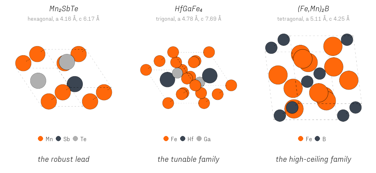
Table 4 collects the leading candidates, and Figure 10 shows the screened cells behind the three rare-earth-free families. A manufactured magnet, however, is a polycrystal, and the properties a user sees depend on grain size, grain alignment, and grain-boundary chemistry as much as on the cell itself (Figure 5). For every gate-passing compound the sweep stage therefore tests 2,000 sampled microstructures and records the acceptable window: the region of processing space in which the compound still clears the magnet thresholds (Figure 11).

Table 4. Leading candidates from the screen, with the L1₀ FePt benchmark as the precious-metal reference. Robustness is the share of 2,000 sampled microstructures that clear all magnet thresholds, weighted by their margin above them; the peak energy product is the sweep’s best case. Sintered Nd–Fe–B delivers ≈400 kJ/m³.

compound	family	κ (corr)	$M_s$ (MA/m)	$T_c$ (K)	$E_{hull}$ (meV)	peak $(BH)_{max}$ (kJ/m³)	robustness	note
FePt	L1₀ (precious ref.)	3.15	1.09	538	0	372	0.91	large hardness margin
Mn₂SbTe	layered pnictide-chalcogenide	4.14	0.79	438	4	195	0.71	most robust RE-free lead; FM-assumption flag
HfGaFe₄	trigonal A-Fe	1.77	0.79	545	69	198	0.10	A-site and anion both tunable
ZrGaFe₄	trigonal A-Fe	1.51	0.82	531	78	211	0.05	Zr cheaper than Hf
Fe₇MnB₄	(Fe,Mn)₂B boride	1.11	1.14	650	16	404	0.01	NdFeB-class ceiling, fragile
Fe₁₅MnB₈	(Fe,Mn)₂B boride	1.08	1.18	610	8	423	0.008	highest RE-free ceiling in the set
Mn₂Ge	hexagonal	1.13	1.12	504	51	393	0.01	FM-assumption flag

Ball-and-stick unit cells of Mn2SbTe, HfGaFe4, and (Fe,Mn)2B — **Figure 10.** The screened cells behind Table 4's three rare-earth-free families, drawn from the dataset's structure files. Left: Mn₂SbTe, a layered hexagonal cell in which Mn planes (orange) alternate with Sb (dark gray) and Te (light gray); the stacking supplies the anisotropy that makes it the most robust lead. Center: HfGaFe₄, the trigonal A-Fe motif, an iron framework (orange) with an A site (Hf, dark gray) that flips the easy axis from plane to c and an anion site (Ga, light gray) that tunes the hardness. Right: the tetragonal (Fe,Mn)₂B parent cell (boron in dark gray); substituting one iron site with Mn in a supercell of this structure produces the Fe₁₅MnB₈ and Fe₇MnB₄ leads.

Figure 11. The microstructure windows behind Table 4, from the 2,000-point sweep. FePt's hardness margin (κ ≈ 3) tolerates 40% chemical disorder and any grain size from 10 to 500 nm, which is why L1₀ magnets are manufacturable. Mn₂SbTe is the closest rare-earth-free analogue: a wide window at a moderate 195 kJ/m³ ceiling. Fe₁₅MnB₈ is the opposite corner: an NdFeB-class 423 kJ/m³ ceiling that exists only at a single sampled point (perfect chemical order, exactly 50 nm grains, near-zero grain-boundary exchange), with coercivity the limiting metric in 100% of failing microstructures.

Two rare-earth-free archetypes emerge. The Mn-hardened borides pair iron-rich magnetization with κ barely above one, so their NdFeB-class ceilings survive only under near-perfect processing, with coercivity the limiting metric in every failing microstructure; the high-κ leads (Mn₂SbTe, the A-Fe family) have hardness to spare but half the magnetization. Section 4.4 shows this trade across the whole dataset. Mn₂SbTe and Mn₂Ge carry the ferromagnetic-assumption flag (Section 6), and every value here carries the Section 5 error bars.

4.4 The property landscape

Figure 12 plots every reliable label on the hardness-magnetization plane, and the upper-right corner (compounds simultaneously hard, κ > 1, and strong enough for an NdFeB-class energy-product ceiling, $M_s$ above ~1.13 MA/m) is nearly empty. Iron-rich intermetallics crowd the strong-but-soft left edge; the hard right side belongs to dilute-moment oxides, chalcogenides, and halides. The two Pareto frontiers make the discovery gap quantitative: through the magnet-relevant range the precious-metal frontier (FePt, Fe₃Pt) dominates the precious-free one, and the free frontier’s knee, where hardness and magnetization are best simultaneously, is the (Fe,Mn)₂B boride family of Section 4.3, which touches the ceiling line at κ ≈ 1.

Figure 12. Every κ-reliable label on the hardness-magnetization plane (2,044 compounds, overlapping points merged). Iron-rich intermetallics crowd the strong-but-soft left edge; the hard right side is populated by dilute-moment oxides, chalcogenides, and halides, with the palest points in the flagged-outlier tail. The staircases trace Pareto frontiers over unflagged easy-axis compounds: the precious-metal frontier (dashed) dominates the precious-free frontier (orange) through the magnet-relevant range, and the free frontier crosses the NdFeB-ceiling line only at the κ ≈ 1 boride corner. The nearly empty upper right is the region a rare-earth-free NdFeB replacement must occupy.

A permanent magnet must satisfy three intrinsic requirements at once, and Figure 13 adds the third: the Curie temperature. The three-dimensional Pareto set over hardness, magnetization, and Curie temperature holds 28 compounds, and the added axis reorders the shortlist. High-Curie cobalt-rich compounds (Co₃Cu, FeNi₃, MnCo₄) enter the frontier on thermal margin, while Mn₂SbTe, robust in the two-dimensional planes, drops out: its 438 K Curie point is dominated. The borides survive on all three axes.

Figure 13. The dataset in the three intrinsic dimensions a magnet must satisfy at once: hardness (log κ), magnetization, and Curie temperature. Orange stems mark the 28 compounds that are Pareto-optimal in all three, projected onto the κ-Tc floor for readability. The dashed floor line is κ = 1. The conjunction thins the candidate list further than either two-dimensional view: Mn₂SbTe falls off this frontier (Curie point too low), the (Fe,Mn)₂B borides stay on it, and the high-Curie end belongs to cobalt-rich soft compounds that lack a hardening mechanism.

Figure 14 splits the hardness-magnetization plane by anion class, and each class occupies its own region: intermetallics fill the strong-but-soft upper left, the anion-bearing classes trade magnetization for anisotropy along the lower right, and the borides sit alone in the crossing zone where both are moderate, which is why that family keeps appearing in Section 4.3.

Figure 14. The hardness-magnetization plane split by chemistry class (orange, one panel per class) against the full cloud (gray). The classes cluster: metallic bonding buys magnetization at the upper left, anion chemistry (oxides, chalcogenides, halides) buys anisotropy at dilute moments toward the lower right, and pnictides sit between. The 37 borides straddle the κ = 1 line at high magnetization, the region every other class avoids, marking interstitial boron hardening of an iron-rich lattice as the dataset's distinctive rare-earth-free design route.

Figure 15 repeats the analysis with the engineering pair: the peak energy product against the robustness score, for the 641 compounds that passed every gate. Nearly every compound sits close to one of the two axes. Rare-earth-free compounds reach NdFeB-class ceilings only at robustness near zero (the borides), or usable robustness at half the ceiling (Mn₂SbTe); the approach to the open corner is made only by precious-metal compounds, FePt nearest. No physical bound excludes the corner; it is where a rare-earth-free discovery would land, and the dataset states what occupying it requires: κ comfortably above one and $M_s$ above ~1.1 MA/m in the same uniaxial, stable, high-Curie compound.

Figure 15. The engineering trade for the 641 gate-passing compounds: peak energy product against robustness. High ceilings occur at near-zero robustness (the borides, upper left) and usable robustness at moderate ceilings (Mn₂SbTe); only precious-metal compounds approach the open corner. Fe₃Pt's 706 kJ/m³ ceiling comes with Invar caveats (Section 5.1), which leaves FePt as the appropriate reference point.

5 Technical validation

Screening-scale settings trade accuracy for throughput, and the calibration tier measures how much accuracy is given up. A stratified subset of 287 compounds (roughly fifty per hardness band, interleaved so partial completion stays balanced) was recomputed with the k-point spacing tightened from 0.16 to 0.10 Å⁻¹ and the plane-wave cutoff raised from 65 to 80 Ry, a refinement that costs six to ten times the production runtime per compound. Comparing the two values for the same compound separates the error into a bias and a scatter, and the two behave very differently.

Figure 16. The 287 calibration pairs. The spine follows the identity line closely, and the small downward offset at the hard end is the bias of Table 5; the vertical scatter around the line is the per-label noise that dominates the error budget. Axis↔plane classification changes (dark) concentrate among the compounds that move farthest.

Table 5. Per-band calibration, 287 compounds. The correction is the median ratio of high-accuracy to production $\kappa$; the interquartile range (IQR) is the per-label scatter around it; the flip rate is the fraction whose easy-axis classification (axis vs plane) changed under refinement.

κ band	n	κ correction (median)	IQR	axis↔plane flip
< 0.8	88	×1.002	[0.96, 1.31]	19%
0.8 – 1.2	51	×0.992	[0.90, 1.09]	14%
1.2 – 2	50	×0.983	[0.84, 1.19]	14%
2 – 4	48	×0.963	[0.75, 1.03]	8%
> 4	50	×0.968	[0.79, 1.02]	16%

Figure 17. The calibration result in one picture. The medians (thick lines) hug the no-change line: the systematic bias is 0–4% and grows mildly with hardness. The boxes (interquartile ranges) do not; a typical individual label moves by ±16% under refinement, and the 5–95% whiskers show the heavy tails, largest in the ill-defined soft band. The bias is corrected in the shipped values; the scatter is the irreducible per-label uncertainty and is the number a model trained on this data should be judged against.

The bias is small, κ-dependent, and corrected. The shipped columns kappa_corrected and K1_corrected_J_per_m3 apply each band’s median correction (squared for $K_1$, since $K_1 \propto \kappa^2$ at fixed $M_s$). The correction grows toward the hard end, and the benchmark below shows it grows further for the very hardest compounds, so high-$\kappa$ values should be read as upper estimates.

The scatter is the dominant error term, and it does not average away for a single compound. In the magnet-relevant bands ($\kappa \geq 0.8$, n = 199) the interquartile range of the refinement ratio is [0.84, 1.05], a robust one-sigma of roughly ±16%, with 48% of labels within ±10% of their refined value and 66% within ±25%. In practice, a regression model trained on these labels cannot be validated below a ±15–20% error floor on $\kappa$, because the labels themselves move that much under convergence refinement. Most computed-property datasets report values without a calibration tier; stating the floor lets users size their validation targets correctly.

The easy-axis label is most reliable in the strongly anisotropic bands, where it matters most. The axis↔plane flip rate falls from 19% for soft, nearly-isotropic compounds, where the easy direction is genuinely ill-defined, to 8% in the strongly anisotropic 2–4 band. The shipped easy_axis_confidence column encodes one minus the per-band flip rate.

5.1 Benchmark against literature

Table 6. Computed versus literature $K_1$ (MJ/m³) for canonical hard magnets. “Production” is the as-computed value at screening settings; “refined” is the tightened-settings recomputation, completed for all rows in July 2026; experiment and DFT columns are literature values [12, 13, 19]. The refined easy axis is noted where it differs from production.

compound	easy axis (ours)	$K_1$ production	$K_1$ refined	$K_1$ experiment	$K_1$ DFT literature
FePt (L1₀)	001 ✓	15.9	10.6	~6.6	7–11
FeCoPt₂	001	20.5	10.0	—	10–20
CoPt (L1₀)	001 ✓	8.9	2.5 (→ in-plane ✗)	~4.9	5–8
FePd (L1₀)	in-plane ✗	1.5	1.8 (→ 001 ✓)	~1.8	2–3
Fe₂B	001 ✗	1.4	0.6 (→ plane ✓)	−0.8 (easy-plane)	≈0, near boundary
CrPt, MnPt	non-001	10.4, 6.7	17.7, 8.4	antiferromagnets	—

The pipeline recovers the correct hardness ordering (FePt > CoPt > FePd), and refinement moves the hardest values into the published DFT ranges (FePt 15.9 → 10.6, FeCoPt₂ 20.5 → 10.0 MJ/m³) while they remain above room-temperature experiment, the well-documented gap between zero-temperature density-functional anisotropy and measurement [12, 13]. Refinement also corrects both marginal easy-axis errors: FePd moves from in-plane to the known 001 axis with K1 = 1.8 MJ/m³, matching experiment, and Fe₂B moves from 001 to the easy plane, matching its measured K1 of −0.8 MJ/m³ at room temperature [19]. The Fe₂B result anchors the boride story of Section 4.3 in the literature: the parent compound is easy-plane, and hardening it requires substitution, the role Mn plays in Fe₁₅MnB₈ as Co does in (Fe,Co)₂B alloys [19]. CoPt is the exception, flipping to in-plane against the known easy axis under refinement; single calculations carry the Section 5 per-label variance at either setting, and near-boundary compositions can flip in either direction. The two antiferromagnets, included as controls, fail to present as easy-axis ferromagnets at both settings; their large anisotropy energies are spin–orbit scales, not usable permanent-magnet constants.

6 Usage notes

6.1 Quality flags

Known failure modes of the pipeline are recorded as per-row flags; flagged rows are retained in the dataset, and the filtering threshold is left to the user.

flag	rows	meaning
`kappa_reliable = False`	198	$\kappa = \sqrt{K_1/\mu_0 M_s^2}$ diverges as $M_s \to 0$; near-compensated ferrimagnets produce artifact hardness values (the dataset’s raw maximum, κ ≈ 66, is such an artifact). Flagged when the anisotropy-stage $M_s$ < 0.1 MA/m.
`k1_outlier = True`	165	$K_1$ above 20 MJ/m³ or corrected κ above 8, beyond the credible hard-magnet ceiling (FePt, ~16 MJ/m³ at these settings) and in the calibration tail where single-shot values are least trustworthy. Flagged values should be recomputed at refined settings before use.
`fm_assumption_risk = True`	1,773	The calculation assumes ferromagnetic alignment. Flagged where that plausibly overestimates $M_s$ (hence κ and the energy product): two or more Mn/Cr atoms per formula unit, or multiple magnetic atoms together with an anion, the superexchange chemistry that favors antiferro- or ferrimagnetic order. Half the dataset carries this flag, consistent with its oxide-heavy composition.
`easy_axis_confidence`	all labeled	one minus the per-band axis↔plane flip rate of Table 5.

6.2 Limitations

The dataset is a screening resource, and its limitations follow from that role. Only uniaxial crystal systems are present, so there is no cubic anisotropy data. Ferromagnetic alignment is assumed throughout; true ground-state orderings are not resolved, only flagged. The labels are single calculations at screening settings with the per-label uncertainty of Section 5; the calibration tier quantifies the noise, it does not remove it. Curie temperatures and the derived exchange stiffness are method-level estimates. Absolute anisotropy magnitudes are zero-temperature density-functional values, 1.5–2× room-temperature experiment for hard magnets. Chemistry under-represents nickel-rich compounds, which is at least partly intrinsic, since nickel-rich uniaxial magnets are genuinely scarce. And rare-earth compounds are absent by construction, which is the dataset’s scope, not an oversight: a model trained on it learns the rare-earth-free anisotropy landscape, which is the landscape the discovery problem cares about.

6.3 Intended use

Three uses motivated the construction. The first is training and benchmarking structure-to-anisotropy models against a measured noise floor: the corrected columns are the labels, the calibration tier is a held-out gold standard for uncertainty-aware training, and ±15–20% on $\kappa$ is the error below which validation results measure label noise rather than model skill. The second is screening: the flags plus the corrected values support a screening workflow: require kappa_reliable, recompute k1_outlier rows before use, and treat magnetization-derived figures as upper bounds where fm_assumption_risk is set. The third is negative-example supply: balanced easy-axis/easy-plane and soft/hard populations are rarer in public data than positives, and they are what a classifier needs to learn a decision boundary rather than a density estimate.

Data and code availability

The dataset (v1.0) is available on the Hugging Face Hub at huggingface.co/datasets/willgbryan13/magnet-anisotropy-screening under a CC-BY-4.0 license: the main table in Parquet and CSV, the complete per-record pipeline output, the 2,787 relaxed structures with a record-linked manifest, the 287-pair calibration tier, and the parameter-level methods document. Every row carries a stable record_id. The screening cascade, calibration runner, and correction scripts are maintained in the project repository; the property-calculation routes are hosted on the Ouro platform [16].

Acknowledgements

The anisotropy, relaxation, stability, Curie-temperature, and magnetic-property calculations ran as hosted routes on Ouro; the screening orchestration ran on Modal. Source structures draw on the Materials Project [4]. Structure handling used pymatgen [14]. The GPSK-300 structure-generation work that seeded this project is described in the companion report [15].

References

[1] M. Sagawa et al. New material for permanent magnets on a base of Nd and Fe. J. Appl. Phys. 55, 2083 (1984). DOI:10.1063/1.333572

[2] R. Skomski and J. M. D. Coey. Magnetic anisotropy — How much is enough for a permanent magnet? Scripta Mater. 112, 3 (2016). DOI:10.1016/j.scriptamat.2015.09.021

[3] J. M. D. Coey. Magnetism and Magnetic Materials. Cambridge Univ. Press (2010). DOI:10.1017/CBO9780511845000

[4] A. Jain et al. The Materials Project: A materials genome approach to accelerating materials innovation. APL Materials 1, 011002 (2013). DOI:10.1063/1.4812323

[5] S. V. Gallego et al. MAGNDATA: towards a database of magnetic structures. J. Appl. Cryst. 49, 1750 (2016). DOI:10.1107/S1600576716012863

[6] P. Nieves et al. Database of novel magnetic materials for high-performance permanent magnet development. Comput. Mater. Sci. 168, 109340 (2019). DOI:10.1016/j.commatsci.2019.109340

[7] S. Haastrup et al. The Computational 2D Materials Database: high-throughput modeling and discovery of atomically thin crystals. 2D Mater. 5, 042002 (2018). DOI:10.1088/2053-1583/aacfc1

[8] B. Rhodes et al. Orb-v3: atomistic simulation at scale. arXiv:2504.06231 (2025). arXiv:2504.06231

[9] P. Li et al. Large-scale ab initio simulations based on systematically improvable atomic basis. Comput. Mater. Sci. 112, 503 (2016). DOI:10.1016/j.commatsci.2015.07.004

[10] X. He, N. Helbig, M. J. Verstraete, and E. Bousquet. TB2J: A python package for computing magnetic interaction parameters. Comput. Phys. Commun. 264, 107938 (2021). DOI:10.1016/j.cpc.2021.107938

[11] M. J. van Setten et al. The PseudoDojo: Training and grading a 85 element optimized norm-conserving pseudopotential table. Comput. Phys. Commun. 226, 39 (2018). DOI:10.1016/j.cpc.2018.01.012

[12] D. Weller and A. Moser. Thermal effect limits in ultrahigh-density magnetic recording. IEEE Trans. Magn. 35, 4423 (1999). DOI:10.1109/20.809134

[13] A. B. Shick and O. N. Mryasov. Coulomb correlations and magnetic anisotropy in ordered L1₀ CoPt and FePt alloys. Phys. Rev. B 67, 172407 (2003). DOI:10.1103/PhysRevB.67.172407

[14] S. P. Ong et al. Python Materials Genomics (pymatgen): A robust, open-source python library for materials analysis. Comput. Mater. Sci. 68, 314 (2013). DOI:10.1016/j.commatsci.2012.10.028

[15] W. Bryan. GPSK-300: A Reciprocal-Space Diffusion Model for L1₀ Magnet Structure Prediction. ghost-projects (2026). /project-014/gpsk-300/

[16] Ouro Foundation. Hosted property-prediction routes for materials science. ouro.foundation

[17] S. Curtarolo et al. AFLOW: An automatic framework for high-throughput materials discovery. Comput. Mater. Sci. 58, 218 (2012). DOI:10.1016/j.commatsci.2012.02.005

[18] H. Sahasrabuddhe, J. Zheng et al. A High-Throughput ab initio Database of Harmonic Phonon Properties for Inorganic Crystals. ChemRxiv preprint (2026). DOI:10.26434/chemrxiv.15004632

[19] A. Edström, M. Werwiński, D. Iuşan, J. Rusz, O. Eriksson, K. P. Skokov, I. A. Radulov, S. Ener, M. D. Kuz’min, J. Hong, et al. Magnetic properties of (Fe1−xCox)2B alloys and the effect of doping by 5d elements. Phys. Rev. B 92, 174413 (2015). DOI:10.1103/PhysRevB.92.174413

flag	rows	meaning
`kappa_reliable = False`	198	\(\kappa = \sqrt{K_1/\mu_0 M_s^2}\) diverges as \(M_s \to 0\); near-compensated ferrimagnets produce artifact hardness values (the dataset’s raw maximum, κ ≈ 66, is such an artifact). Flagged when the anisotropy-stage \(M_s\) < 0.1 MA/m.
`k1_outlier = True`	165	\(K_1\) above 20 MJ/m³ or corrected κ above 8, beyond the credible hard-magnet ceiling (FePt, ~16 MJ/m³ at these settings) and in the calibration tail where single-shot values are least trustworthy. Flagged values should be recomputed at refined settings before use.
`fm_assumption_risk = True`	1,773	The calculation assumes ferromagnetic alignment. Flagged where that plausibly overestimates \(M_s\) (hence κ and the energy product): two or more Mn/Cr atoms per formula unit, or multiple magnetic atoms together with an anion, the superexchange chemistry that favors antiferro- or ferrimagnetic order. Half the dataset carries this flag, consistent with its oxide-heavy composition.
`easy_axis_confidence`	all labeled	one minus the per-band axis↔plane flip rate of Table 5.

Ghost Projects