GPSK-300: A Reciprocal-Space Diffusion Model for L1₀ Magnet Structure Prediction

GPSK-300

Will Bryan · ghost-projects · May 2026

Abstract

We present GPSK-300, a 302M-parameter multimodal diffusion transformer that generates inorganic crystal structures in reciprocal space rather than real space. Existing generative models predict the unit cell with a learned head, so any lattice error propagates into the final structure. Our representation adds a reciprocal-metric channel whose quadratic form determines the six lattice parameters exactly: a linear least-squares fit recovers the lattice from the model output, and an inverse Fourier transform recovers the atomic positions, with no learned geometry head. Closed-form recovery is therefore exact, ≈0% lattice error against 7.7% for the learned head it replaces.

On a permanent-magnet benchmark, GPSK-300 recovers the trained L1₀ tetragonal magnets within ±4% on both lattice constants and produces each candidate in about five seconds, against the hours to days classical crystal structure prediction (CSP) requires. A controlled holdout fixes the limits of this reliability: unseen compositions within a trained family recover at nearly the trained rate (≈48% versus ≈58% exact structure match), and unseen intermetallics recover up to quaternary Heuslers, while an entirely unseen structural family is not recovered until a handful of fine-tuning examples teach it. GPSK-300 is best understood as a fast CSP structure proposer for represented motifs, evaluated by per-family recovery against known references rather than by novelty metrics that penalize recovering the right answer.

1 Introduction

Crystal structure prediction (CSP) determines the equilibrium crystal structure that a given chemical composition adopts, and it is a prerequisite for computational materials discovery. The properties that determine whether a composition merits further study, including thermodynamic stability, electronic structure, and magnetic behavior, depend on the arrangement of the atoms and not on the chemical formula alone, so a researcher cannot assess a composition until CSP supplies its structure. Classical CSP methods (USPEX [7], CALYPSO [8], AIRSS [9]) search the space of candidate arrangements and score each one with density functional theory. They produce reliable structures, but each composition requires hours to days of computation, and this cost dominates any campaign that must screen thousands of compositions.

Recent generative models reduce this cost by orders of magnitude, sampling candidate structures directly instead of searching. They differ in the task they address: DiffCSP [26] and FlowMM [27] target crystal structure prediction, while MatterGen [10] and CDVAE [25] target the generation of novel materials. Two problems matter when the goal is CSP. The first concerns evaluation. The prevailing metric for generative crystal models, the Stable–Unique–Novel (SUN) rate, rewards structures that are stable, distinct from one another, and absent from the training set. That goal is the right one for novel-materials generation but the wrong one for CSP: given a known composition, the correct answer is its known structure, so under SUN a model that recovers the real FePt cell counts as “not novel,” and the metric scores it as a failure for being right. The second problem is representational, and it is common to all of these models. They encode the crystal in real space, as fractional atomic coordinates inside an explicit lattice, and produce the lattice with a learned component: CDVAE regresses it from a latent, while MatterGen, DiffCSP, and FlowMM diffuse or flow it jointly with the atomic positions. Any error in the predicted lattice passes straight into the final structure, and the representation offers no way to correct it afterward.

A representation that lets the model output reveal the lattice directly, rather than predict it with a head, removes the second problem. We move generation into reciprocal space. There a crystal is described by its structure factor $F(\mathbf{h})$ on integer Miller indices, which we augment with the reciprocal-metric field $1/d^2(\mathbf{h}) = \mathbf{h}^T G^\ast \mathbf{h}$. This field is a quadratic form, and its six coefficients are exactly the six numbers that define the unit cell. A linear least-squares fit then recovers the lattice from the field, and an inverse Fourier transform recovers the atomic positions from the structure factor. The model never predicts a lattice; it only generates a coherent grid, and arithmetic recovers the geometry. We build this representation into GPSK-300, a 302M-parameter multimodal diffusion transformer that we train with rectified flow matching on a curated corpus of 2,000,115 structures drawn from public DFT and experimental databases. On the trained L1₀ tetragonal magnets (FePt, CoPt, FeNi, MnAl) [3, 4, 5] the model recovers reference structures within ±4% on both lattice constants in roughly five seconds on a single GPU, and it responds to the conditioning signals it learned during training (composition, crystal system, space group, band gap, formation energy, energy above hull, magnetic ordering). A controlled holdout (Section 6.7) identifies the limits of that reliability: held-out compositions inside a trained family recover at nearly the trained rate, and unseen intermetallic compositions reproduce their frameworks up to quaternary Heuslers, while an entirely unseen structural family, the hexagonal CaCu₅ rare-earth–transition-metal (RE-TM) compounds (SmCo₅, YCo₅, CeCo₅) [6], remains unrecovered until a small number of fine-tuning examples teach it.

Two design choices make GPSK-300 suited to CSP rather than to novelty generation: the reciprocal-space representation yields the lattice in closed form, and we evaluate the model by structural recovery rather than by novelty. We report per-family recovery against known reference structures, that is, the fraction of compositions for which the model returns the established structure. The holdout study (Section 6.7) then delineates where a novel candidate can be trusted: within the structural motifs the model represents, and not beyond them.

The contributions of this paper are:

A three-channel reciprocal-space representation for crystals that recovers the lattice in closed form, encoding it as a smooth quadratic field rather than supplying it as metadata or predicting it with a separate learned head, and that reconstructs the atomic basis by inverse FFT while assigning element identity under the composition prompt rather than solving for it independently.
GPSK-300, a 302M-parameter multimodal diffusion transformer that operates in a 16³×128 latent over this representation, trained with rectified flow matching and classifier-free guidance.

The remainder of the paper proceeds as follows. Section 2 reviews related work. Section 3 introduces the structure-factor representation, the reciprocal metric tensor, and the diffusion methods the model builds on. Section 4 describes the encoder, generator, and closed-form decoder. Section 5 covers the training data and protocol. Section 6 reports invertibility, L1₀ magnet recovery, the composition/family holdout, conditioning-modality emergence, and breadth and failure-mode analysis. Section 7 discusses the system’s scope and limits, and Section 8 outlines next steps.

Two parts of the broader permanent-magnet design problem fall outside this work. Synthesizability (whether a tractable physical process can realize a candidate structure) and microstructural engineering (control of grain size, crystallographic texture, domain-wall pinning, and second-phase distributions, which together govern the gap between intrinsic and extrinsic magnetic figures of merit) matter as much as the structure itself for producing a working magnet, and we address neither. GPSK-300 returns a candidate crystal structure for a composition; downstream filtering for thermodynamic stability, synthesis route, and microstructural performance belongs to property-prediction models, multi-scale simulation, and experimental validation.

Classical CSP searches the space of candidate atomic arrangements and ranks them with first-principles energies. USPEX [7] uses evolutionary search, CALYPSO [8] particle-swarm optimization, and AIRSS [9] random sampling, each scored with density functional theory. These methods are reliable and remain the reference standard, but a single composition costs hours to days, which limits high-throughput use.

Generative models replace search with sampling. CDVAE [25] pairs a variational autoencoder with a diffusion decoder and reports reconstruction and de novo generation; MatterGen [10] diffuses atom types, coordinates, and the lattice jointly and conditions on target properties for de novo design; DiffCSP [26] and FlowMM [27] address CSP directly, the former with periodic equivariant diffusion and the latter with Riemannian flow matching, both scoring match rate against reference structures. All four share a representational choice: they encode the crystal in real space and produce the lattice with a learned component, so a lattice error propagates into the final structure. Our reciprocal-space representation removes that dependence.

The generative stage builds on diffusion and flow-matching methods for continuous data. Denoising diffusion [12] and score-based modeling [13] established the framework; flow matching [14] and rectified flow [15] recast it as learning a velocity field along straight paths, which underlies large-scale systems such as Stable Diffusion 3 [16]. GPSK-300 uses rectified flow with classifier-free guidance for few-step sampling and stable training.

GPSK-300 draws on the public crystal databases assembled by the community, including the Materials Project [21], Alexandria [22], OQMD [29], the Crystallographic Open Database [30], and MAGNDATA [31], curated here into a balanced corpus of two million structures. Generative crystal models are most often scored by the Stable–Unique–Novel (SUN) rate and related novelty measures (for example LeMat-GenBench [20]), which suit de novo generation but mismeasure structure prediction, since recovering a known structure counts against a novelty score. We instead report per-family recovery against known references, the measure appropriate to a CSP system.

3 Background

3.1 Structure factors and reciprocal space

A crystal is one arrangement of atoms, the unit cell, repeated periodically through space. Two things specify it. The lattice is the set of six numbers $a, b, c, \alpha, \beta, \gamma$ that fix the size and shape of the repeating box. The basis is the list of atomic positions $\{\mathbf{r}_j\}$ and their chemical species $\{Z_j\}$ inside that box. GPSK-300 does not operate on this real-space description directly. It operates on the crystal’s diffraction pattern, the quantity an X-ray or neutron experiment measures, which represents the same structure in a form that the following sections recover in closed form.

A diffraction pattern labels each scattering direction by a triple of integers $\mathbf{h} = (h, k, l)$, the Miller index, which names a family of parallel planes through the crystal. The structure factor $F(\mathbf{h})$ gives the amplitude and phase the crystal scatters into direction $\mathbf{h}$:

$$F(\mathbf{h}) \;=\; \sum_j f_{Z_j}(s)\,\exp\!\bigl(2\pi i\,\mathbf{h}\cdot\mathbf{r}_j\bigr)$$

The atomic scattering factor $f_{Z_j}(s)$ sets how strongly element $Z_j$ scatters, evaluated at $s = \sin\theta/\lambda = 1/(2d)$, where $d(\mathbf{h})$ is the spacing between the (hkl) planes. Heavier elements hold more electrons and scatter more strongly, so $f$ grows with atomic number; the Cromer–Mann four-Gaussian form [11] captures its dependence on $s$:

$$f_Z(s) \;=\; \sum_{i=1}^{4} a_i^{(Z)}\,e^{-b_i^{(Z)}\,s^2}$$

Element identity therefore shapes the magnitude of $F$ at every Miller index, not only through a single atomic number.

$F$ is generally complex, and $F(-\mathbf{h}) = F(\mathbf{h})^*$ whenever the basis charge density is real. Re F is then even in $\mathbf{h}$, while Im F is odd and vanishes everywhere for a centrosymmetric basis, where every atom at $\mathbf{r}_j$ has a partner at $-\mathbf{r}_j$ and the sine terms cancel in pairs. Inversion symmetry is common, so this constraint holds for a large share of the training set, and the model can use it to simplify what it has to generate.

Figure 1. The model's three input channels are sampled at integer Miller indices. Re F(h) is even with a bright DC term and signed Bragg peaks falling off outward. Im F(h) is odd, vanishes at the origin, and flips sign through inversion. 1/d²(h) is a smooth quadratic, small near the origin, growing radially.

3.2 The reciprocal metric tensor

The structure factor carries the basis. The lattice enters separately, through the plane spacings $d(\mathbf{h})$, and it does so in a way that makes recovery easy. The squared inverse spacing is a single quadratic function of the Miller index:

$$\frac{1}{d^2(\mathbf{h})} \;=\; \mathbf{h}^T G^\ast \mathbf{h} \;=\; g_{11}h^2 + g_{22}k^2 + g_{33}l^2 + 2g_{12}hk + 2g_{13}hl + 2g_{23}kl$$

The matrix $G^\ast = G^{-1}$ is the reciprocal metric tensor, the inverse of the real-space metric tensor $G$ built from the lattice vectors. $G^\ast$ has six independent components, one for each of the six lattice degrees of freedom $(a, b, c, \alpha, \beta, \gamma)$, so recovering these six numbers recovers the lattice. Evaluated over a 64³ Miller-index grid, the quadratic gives one equation per grid point, roughly 262,000 equations for six unknowns. Recovering the lattice is therefore a linear least-squares fit, with no learned component and no sensitivity to noise in any single value.

Figure 2. In a centrosymmetric basis (left) every atom at r has a partner at −r through the inversion center (dashed pairings), and the sine terms in F(h) = Σ f_j exp(2πi h·r_j) cancel pairwise, so Im F vanishes. An asymmetric basis (right) has no such pairings, so Im F survives at every hkl.

Figure 3. The 1/d²(h) iso-contours take a different shape for each crystal system: cubic is rotationally symmetric (a=b=c), the L1₀ tetragonal family stretches along one axis (a=b≠c), and monoclinic tilts the principal axes (β≠90°). The shape of the iso-contour ellipsoid directly encodes the lattice metric.

3.3 Diffusion models and rectified flow matching

A generative model learns to turn random noise into samples that resemble its training data. Modern continuous-data models do this gradually: they define a path that connects a simple noise distribution $p_0$ (here, Gaussian noise) to the data distribution $p_1$, and they learn how to move a sample along that path one small step at a time [12]. Score-based diffusion [13] learns the path through the score $\nabla_x \log p_t(x)$, the direction toward higher data density at each intermediate point. Flow matching [14] learns it more directly, as a velocity field $v_\theta(x, t)$ that the model trains to match a chosen target velocity.

Rectified flow [15] is the special case where the path between a paired noise sample and data sample $(x_0, x_1)$ is a straight line:

$$x_t \;=\; (1-t)\,x_0 \,+\, t\,x_1, \qquad v^\star \;=\; x_1 - x_0$$

and the training objective collapses to a constant target along each path:

$$\mathcal{L}(\theta) \;=\; \mathbb{E}_{t,\,x_0,\,x_1,\,c}\!\left[\,\bigl\|\,v_\theta(x_t, t, c) \,-\, (x_1 - x_0)\,\bigr\|^2\,\right]$$

At inference we integrate this velocity field as an ODE $\dot{x} = v_\theta(x, t)$ from $t = 0$ to $t = 1$, and because the trajectories are straight by construction, a small number of Euler steps suffices. This formulation underlies recent large-scale image and video generators including Stable Diffusion 3 [16], and it forms GPSK-300’s diffusion stage.

Figure 4. Each noise sample x₀ pairs with a data sample x₁, and the model v_θ learns to predict the constant velocity v⋆ = x₁ − x₀ at every t along the segment between them. The target is independent of the position along the path, which makes the objective easier to optimize than score matching.

To amplify conditioning at inference, GPSK-300 applies classifier-free guidance [17]. The model learns to predict both the conditional velocity $v_\theta(x_t, t, c)$ and the unconditional velocity $v_\theta(x_t, t, \varnothing)$, because training randomly drops the conditioning on some examples, and at inference we extrapolate past the conditional velocity:

$$\tilde{v}_\theta(x_t, t, c) \;=\; v_\theta(x_t, t, \varnothing) \,+\, w\,\bigl(\,v_\theta(x_t, t, c) - v_\theta(x_t, t, \varnothing)\,\bigr)$$

With $w = 1$ this reduces to ordinary conditional sampling; for $w > 1$ the model is pulled more strongly in the direction the conditioning would already have pulled it, trading sample diversity for stronger response to $c$. This setting matters more than usual for continuous-property conditioning: without it the model averages over the data distribution and ignores the property entirely.

4 Method

The pipeline has five stages, and the rest of this section takes them in order. We first turn each crystal into a three-channel reciprocal-space grid (Section 4.1). A small VAE compresses that grid into a compact latent (Section 4.2). A diffusion transformer learns to generate latents from noise under the conditioning signals (Section 4.3), trained with rectified flow matching (Section 4.4). At inference we sample a latent and decode it back to a grid (Section 4.5), then read the crystal structure out of the grid by arithmetic (Section 4.6). Figures 5a and 5b show the full path from noise to structure.

4.1 Representation

We represent each crystal as a $64^3 \times 3$ tensor sampled on the integer Miller-index grid $(h, k, l) \in [-32, 31]^3$. The three channels are:

$$X(\mathbf{h}) \;=\; \bigl(\,\mathrm{Re}\,F(\mathbf{h}),\; \mathrm{Im}\,F(\mathbf{h}),\; 1/d^2(\mathbf{h})\,\bigr).$$

The first two channels carry the basis: the atomic positions and, through the Cromer–Mann scattering factors, the element identities. The third channel carries the lattice geometry as its quadratic form.

Three choices in how we store these channels matter for recovering the structure later. First, we compress the structure-factor magnitudes by an exponent γ = 0.5 (|F| → |F|^γ, which keeps the phase) before storing them. A few Bragg peaks are far brighter than the rest, and without compression the VAE and flow model would spend their capacity on those peaks alone; compression spreads the values out so the model represents the whole pattern, and we invert the exponent at decode. Second, we divide F by its per-sample maximum magnitude and keep that maximum, norm_factor = max|F|, for the inverse transform; this preserves the relative pattern without encoding the absolute electron count. Third, we divide the 1/d² channel by a fixed constant, INV_D2_NORM = 200 Å⁻², rather than a per-sample value. A fixed divisor keeps the absolute lattice scale in the channel values themselves, so the closed-form lattice recovery reads it from the grid and needs no separate per-sample metadata.

4.2 Encoder VAE

A small 3D convolutional VAE ($\approx$2.6M parameters) maps the $64^3 \times 3$ grid to a $16^3 \times 128$ latent, shrinking the spatial size by a factor of four per axis while widening the channels. The 1/d² channel is a smooth quadratic over a regular grid, so the VAE encodes it almost losslessly, reaching a reconstruction MSE near $10^{-6}$ on held-out structures. The structure-factor channels are sparse, since most of the amplitude sits near the origin, but the VAE handles them well enough at this resolution, and we needed no per-channel specialization.

4.3 MMDiT generator

The generator is a multimodal diffusion transformer (MMDiT, ≈302M parameters) operating on the 16³×128 latent. Each block is double-stream: image tokens (sequenced from the spatial latent) and conditioning tokens (composition, crystal system, space group, band gap, formation energy, energy above hull, magnetic ordering) attend jointly through a shared attention mechanism [19], allowing conditioning tokens to attend to specific spatial regions of the latent rather than only modulating activations globally. AdaLN-Zero modulation [18] on every block provides an additional global conditioning signal initialized so that residual blocks start as identity, which stabilizes training at this scale. After the double-stream blocks, the model passes into single-stream blocks operating on the merged token sequence.

4.4 Training: rectified flow matching

We take a data latent $z_1 \sim p_\text{data}$ and an isotropic Gaussian sample $z_0 \sim \mathcal{N}(0, I)$, and interpolate between them along a straight line:

$$z_t \;=\; (1-t)\,z_0 + t\,z_1, \qquad t \sim \mathcal{U}(0,1)$$

The model then learns to predict the constant velocity that carries noise to data, minimizing the rectified-flow objective from Section 3.3:

$$\mathcal{L}(\theta) \;=\; \mathbb{E}_{t,\,z_0,\,z_1,\,c}\!\left[\,\bigl\|\,v_\theta(z_t, t, c) - (z_1 - z_0)\,\bigr\|^2\,\right]$$

During training we drop each conditioning token group $c$ with probability $p_\text{drop} = 0.1$, so the one network learns both the conditional and the unconditional velocity field, which inference needs for classifier-free guidance (Figure 4). Training ran for 500k optimization steps on the GPSK-Inorganic-Crystals corpus [28], and the deployed model is the 400k-step checkpoint, which we select on held-out recovery (Section 6.7). Section 5 gives the full source breakdown and curation procedure.

4.5 Inference

Sampling integrates the ODE $\dot{z} = v_\theta(z, t)$ from $t = 0$ to $t = 1$ with 50 forward Euler steps. At every step, classifier-free guidance amplifies the conditioning signal:

$$\tilde{v}_\theta(z_t, t, c) \;=\; v_\theta(z_t, t, \varnothing) \,+\, w\,\bigl(\,v_\theta(z_t, t, c) - v_\theta(z_t, t, \varnothing)\,\bigr)$$

The default guidance scale is $w = 6.0$, substantially higher than typical image-generation values. The dominant signal that needs amplification is property-conditioning on continuous values (formation energy, band gap, energy above hull); at $w \le 1$ the model averages over the data distribution and the property conditioning has no measurable effect on the output, while at $w \approx 6$ the response curves are monotonic in the conditioning value (Section 6.4). Lattice recovery prefers gentler guidance, so the structural evaluations use $w \approx 3$ (Figure 12). End-to-end sampling takes approximately five seconds per candidate on a single GPU.

Figure 5a. A Gaussian noise sample z₀ is integrated through 50 Euler steps of the conditional rectified-flow ODE with classifier-free guidance at w = 6, producing the data latent z₁. The VAE decoder maps that latent back to a 64³ × 3 reciprocal-space grid, and the closed-form decoder of Section 4.6 turns the grid into a pymatgen Structure. The conditioning input c enters the MMDiT directly; its internal routing through the network is detailed in Figure 5b. End-to-end inference takes approximately five seconds per candidate.

Figure 5b. The seven conditioning streams are each tokenized, individually dropped during training with p_drop = 0.1, and fed as a separate token stream into the MMDiT's double-stream blocks, where they attend jointly with the latent image tokens. The MMDiT (≈302M params) processes the latent through a linear projection, N double-stream blocks (joint attention plus AdaLN-Zero), M single-stream blocks (merged self-attention plus AdaLN-Zero), and a linear output head producing the velocity field v_θ. The VAE decoder (≈2.6M params) is a cascade of 3D transposed convolutions upsampling the 16³ × 128 latent to a 64³ × 3 grid, terminating in a 1×1×1 channel projection.

Figure 6. At a single inference step, v_∅ is the unconditional velocity and v_c the conditional velocity. The guided velocity ṽ lies on the line through the two tips (dashed) and extrapolates past v_c when w > 1, magnifying the conditional direction.

4.6 Closed-form decode

Once the model produces a $64^3 \times 3$ grid, reconstruction is closed-form.

Atom positions come from the structure-factor channels: combine channels 0 and 1 into a complex field $F = \mathrm{Re}\,F + i\,\mathrm{Im}\,F$, inverse FFT, and take $|\cdot|$ to obtain the fractional electron density $\rho(\mathbf{r})$. Periodic-aware peak finding with a minimum-separation criterion gives candidate atomic sites. The detection step over-samples with a low threshold and then keeps the top-$N$ peaks, $N = n_\text{f.u.} \cdot \sum_e \nu_e$, where the formula-unit count is selected jointly from the cell volume and the peak intensities. Candidate counts are bounded to a physical per-atom-volume window (8–40 Å³ per atom, spanning dense intermetallics through large ionics):

$$\Bigl\lceil V_\text{cell} \,/\, \bigl(40\,\text{Å}^3 \cdot \textstyle\sum_e \nu_e\bigr) \Bigr\rceil \;\le\; n_\text{f.u.} \;\le\; \Bigl\lfloor V_\text{cell} \,/\, \bigl(8\,\text{Å}^3 \cdot \textstyle\sum_e \nu_e\bigr) \Bigr\rfloor$$

and within the window the count with the largest drop in ranked peak intensity is selected, since true atomic peaks are bright and spurious ones dim. For dense small cells the window collapses to a single candidate; for large-volume-per-atom ionics the intensity gap resolves the count. This enforces requested stoichiometry exactly.

The lattice comes from channel 2: denormalize to recover $1/d^2(\mathbf{h})$ on the integer grid, then assemble the design matrix $\mathbf{A} = [\,h^2,\,k^2,\,l^2,\,2hk,\,2hl,\,2kl\,]$ over all non-origin grid points and solve the linear least-squares problem $\min_{\mathbf{g}} \|\mathbf{A}\mathbf{g} - \mathbf{y}\|^2$ for the six independent components of $G^\ast$. Invert $G^\ast \to G$ and read off:

$$a = \sqrt{G_{11}},\; b = \sqrt{G_{22}},\; c = \sqrt{G_{33}}, \quad \cos\alpha = G_{23}/(bc),\; \text{etc.}$$

Composition is assigned last: the deployed decoder assumes the requested formula and maps heavier elements to brighter peaks. The heuristic recovers element identity correctly because the Cromer–Mann scattering magnitude scales monotonically with atomic number, and it remains robust even for near-Z neighbors (Fe/Co/Ni, Mn/Fe). It reads density peak heights, which the inverse FFT concentrates at atomic sites, so they are stable under reconstruction error: across encoded near-Z binaries, the heuristic assigns elements correctly at 100% both noise-free and under the VAE’s own round-trip error (Figure 8). The reliability is binary-specific, however: with three or more species on distinct sublattices, near-Z pairs are confused more often (NiMnSb in Section 6.8), and disambiguation beyond binaries remains open (Section 8). A magnitude-fitting alternative (joint Cromer–Mann least squares) is exact in the noise-free limit but less robust: it overfits the reconstruction error to neighboring atomic numbers and drops to ~60% on the same near-Z cases, so the simple heuristic is retained.

Figure 7. The two structure-factor channels combine into a complex field, are inverse-FFT'd to a fractional electron density, and peak-found to recover atom positions. The reciprocal-metric channel is fit by linear least squares to recover G*, which is inverted to read off the six lattice parameters. The two streams merge into a pymatgen Structure. No learned post-processing.

Figure 8. Element-identity accuracy on near-Z pairs (Fe/Co/Ni, Mn/Fe) holds for the brightness heuristic but not for a Cromer–Mann magnitude fit as reconstruction error increases. Both are exact on clean and white-noise-perturbed inputs, but under realistic VAE reconstruction error the magnitude fit overfits the error to neighboring atomic numbers and degrades, while the heuristic, reading inverse-FFT peak heights, remains exact. The heuristic is therefore retained in the deployed decode.

5 Experimental Setup

5.1 Dataset

We train GPSK-300 on the GPSK-Inorganic-Crystals dataset [28], 2,000,115 structures drawn from LeMat-Bulk [20], Materials Project [21], Alexandria [22], OQMD [29], the Crystallographic Open Database [30], and MAGNDATA [31]. We deduplicate by entalpic fingerprint and balance the set jointly across space group, number of sites, and chemical family, which preserves the long tail of rare structural families (L1₀ tetragonal, hexagonal RE-TM, cubic perovskite, rock-salt oxide). For the held-out generalization study (Section 6.7), we exclude a 0.31% slice before precomputing the representation, namely the entire hexagonal RE-TM family together with the FePd and MnGa compositions, and keep everything else. We then compute the three-channel representation for each structure following Section 4.1.

5.2 Conditioning

The model takes seven conditioning streams: composition, crystal system, space group, band gap, formation energy per atom, energy above hull, and magnetic ordering. We embed each stream separately and drop it independently with probability 0.1 during training, so a user can supply any subset at inference. Composition needs care in particular. An early ablation showed that the standard pymatgen reduced_formula is ambiguous: “NaCl” could mean the 2-atom cell or the 8-atom cell, and the model could not tell them apart. The deployed model instead uses raw atom counts (“Na1 Cl1” versus “Na4 Cl4”), which makes multi-formula-unit prompts distinguishable in the generated structures and measurably improves per-family lattice accuracy.

5.3 Training and inference

We train in stages. First we precompute the three-channel grids once and cache them as parquet. Then we train the VAE to convergence and freeze it, which stops the diffusion model from absorbing encoder noise during its own optimization. Finally we train the MMDiT for 500k optimization steps with AdamW on the rectified-flow loss over the cached latents.

At inference we integrate the flow ODE with 50 forward Euler steps and classifier-free guidance, then keep the best of N candidates. The guidance scale depends on the task (Section 6.4): structural evaluations use $w \approx 3$, the lattice-recovery optimum, while property-conditioning sweeps use the $w = 6$ serving default. N also varies by experiment, with 10 candidates per prompt for the magnetic evaluation, 16 for the L1₀ recovery in Table 1, and 48 for the holdout study (Section 6.7); in each case we report the closest match to reference.

6 Results

6.1 Invertibility

We first verify the round-trip: take a known structure, encode it to the three-channel grid, decode immediately, and compare. On a held-out set of test structures the encoded-then-decoded structure matches the source to roughly 4 decimal places on every lattice parameter (worst-case ≤ 0.0005 Å on edge lengths and ≤ 0.05° on angles), and atomic positions land within 0.01 fractional coordinate of the reference. With the trained VAE inserted into the round-trip (encode to grid, VAE encode and decode, then decode to structure), end-to-end correlation with the source grid is 99.9%. The lattice channel alone reconstructs to MSE $\sim 10^{-6}$, and the closed-form lattice recovered from the VAE-reconstructed grid stays within ~0.3% of the source edges.

6.2 L1₀ tetragonal family

The L1₀ family is a primary target for rare-earth-free permanent magnets: tetragonal P4/mmm intermetallics with alternating A/B atomic planes along the c axis. (Two cell conventions coexist for L1₀: the conventional face-centered description has c/a just under unity, while the primitive tetragonal cell used throughout this paper, whose a is smaller by √2, has c/a ≈ 1.37.) The four trained members, FePt, CoPt, FeNi, MnAl, recover to within ±4% on both $a$ and $c$ (Table 1, best-of-N selection with N = 16); we hold two further members, FePd and MnGa, out of training, and both recover at nearly the same rate (Section 6.7). The c/a ratio is the most important structural number for L1₀ magnets because it controls the magnetocrystalline anisotropy that makes these compounds useful, and the model preserves it to within ~3% across the family.

Table 1. L1₀ tetragonal magnet recovery (trained members; best-of-N selection with N = 16). Reference parameters from published crystallography [3, 4, 5]. Ratios are recovered/reference; values near 1.00 are best.

Composition	ref a (Å)	ref c (Å)	a ratio	c ratio	family role
FePt	2.73	3.73	0.995	1.003	classic FePt, K₁ ≈ 7 MJ/m³
CoPt	2.68	3.70	0.986	1.017	high anisotropy
FeNi	2.53	3.58	0.987	0.985	tetrataenite, RE-free
MnAl	2.78	3.56	0.965	0.998	τ-MnAl RE-free

Generated versus expected crystal structures across the model's range: recovered L1₀ magnets, metals, rock-salt, fluorite, and zinc-blende prototypes; held-out compositions; ternary and quaternary intermetallics absent from the corpus; and characteristic failures. — **Figure 9a.** GPSK-300's outputs span the model's range, from recovered families to characteristic failures, each shown as the generated crystal beside the expected reference at a common scale. The recovered group covers the L1₀ magnets, the simple metals, the rock-salt ionics (MgO, LiF, NaCl), fluorite, and the zinc-blende covalents; held-out compositions (FePd, MnGa) recover at nearly the seen rate; and intermetallics absent from the corpus under their own formulas interpolate the same way: Co₂MnSi and the quaternary CoFeMnSi recover the Heusler cell, while NiMnSb produces the correct half-Heusler framework with the near-Z Ni/Mn pair swapped. The off-target cases are visible directly: the unseen hexagonal family produces a tall cell rather than the squat CaCu₅ geometry; KCl, CsCl, the perovskite, the chalcopyrite, and the kesterite generate coherent but structurally wrong cells; and the large cells (LiFePO₄, Nd₂Fe₁₄B) return full-size cells whose atomic positions lose precision as the cell grows (Section 6.9). Per-structure metrics are in Tables 1–4 and Appendix A.

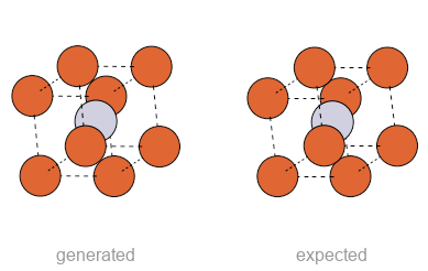
**Figure 9a.** GPSK-300's outputs span the model's range, from recovered families to characteristic failures, each shown as the generated crystal beside the expected reference at a common scale. The recovered group covers the L1₀ magnets, the simple metals, the rock-salt ionics (MgO, LiF, NaCl), fluorite, and the zinc-blende covalents; held-out compositions (FePd, MnGa) recover at nearly the seen rate; and intermetallics absent from the corpus under their own formulas interpolate the same way: Co₂MnSi and the quaternary CoFeMnSi recover the Heusler cell, while NiMnSb produces the correct half-Heusler framework with the near-Z Ni/Mn pair swapped. The off-target cases are visible directly: the unseen hexagonal family produces a tall cell rather than the squat CaCu₅ geometry; KCl, CsCl, the perovskite, the chalcopyrite, and the kesterite generate coherent but structurally wrong cells; and the large cells (LiFePO₄, Nd₂Fe₁₄B) return full-size cells whose atomic positions lose precision as the cell grows (Section 6.9). Per-structure metrics are in Tables 1–4 and Appendix A.

Three independent generated samples each for FePt, MgO, Co2MnSi, and SmCo5, showing recovery and off-target behavior are both consistent across samples. — **Figure 9b.** The behavior in Figure 9a is typical across samples, not a cherry-picked best-of-N. Three independent generations appear for a recovered metal magnet (FePt), a recovered rock-salt oxide (MgO), a ternary Heusler absent from the corpus under its own formula (Co₂MnSi), and the held-out hexagonal family (SmCo₅). Every FePt sample returns the L1₀ tetragonal motif and every MgO sample the rock-salt cell; Co₂MnSi returns the Heusler cell in half of its samples despite the composition never appearing in training; and every SmCo₅ sample is tall rather than the squat CaCu₅ geometry. Recovery and off-target behavior are both reproducible, not artifacts of selecting the best of many tries.

6.3 Hexagonal rare-earth–transition-metal magnets

The CaCu₅-type hexagonal RE-TM structures (space group P6/mmm) are the second key magnetic family, and they serve as the family-level arm of the holdout study (Section 6.7): we exclude the entire hexagonal RE-TM family from training (Section 5.1). On this held-out family the model does not reproduce the squat CaCu₅ geometry: across SmCo₅, YCo₅, and CeCo₅ it defaults to tall cells (generated c/a ≈ 1.3–1.6 in the Table 2 run, and tall in every replicate across runs, against the squat target ≈ 0.80), a 0% structure-match rate (Table 2). This is the negative control that validates the holdout methodology, the case designed to fail, confirming the holdout removed the information it was meant to remove: the model’s default for hexagonal prompts, learned from non-RE-TM hexagonal structures that are predominantly tall, stays tall when asked for a squat motif it never saw.

Table 2. Held-out hexagonal RE-TM family, deployed model, never trained on this family. Squat CaCu₅ target c/a ≈ 0.80.

Composition	target c/a	generated c/a	structure-match
SmCo₅	0.79	≈1.6	✗ (0/10)
YCo₅	0.81	≈1.5	✗ (0/10)
CeCo₅	0.82	≈1.5	✗ (0/10)

This family-level failure is not permanent, however. Fine-tuning the trained model on a small number of squat CaCu₅ examples reverses the tall default: as few as one to five examples move all three targets into the correct squat regime (c/a ≈ 0.88, recovered in 8–10 of 12 samples), and the recovery is stable as more are added (Figure 10). The unseen motif is reachable: the base model is already capable of producing it, and a small number of the right examples is enough to teach it. Acquiring a new family is therefore a small post-training cost, not a full retraining run. The fine-tuning set must be curated to the target motif, since the broad RE-TM pool is dominated by tall hexagonal structures and does not teach the squat one; the metric here is the lattice c/a, the defining squat signature, rather than a full structure match.

Figure 10. The median c/a of generated SmCo₅/YCo₅/CeCo₅ falls toward the squat target as the number of squat-CaCu₅ fine-tuning examples K grows. The base model (K = 0) generates tall cells (c/a ≈ 1.8) far from the target; a single curated example shifts generation into the squat regime (c/a ≈ 0.88, near the 0.80 target), and the recovery is stable as K grows.

6.4 Conditioning modality emergence

For each modality, we tracked the correlation between requested conditioning value and the measured value in the generated structure (or, for categorical conditioning, the fraction of samples respecting the requested label) across the training schedule. Each modality shows a clear emergence checkpoint where the signal moves from indistinguishable from noise to strong, and the order runs counter to the naive expectation: symmetry information appears first, continuous properties last (per-modality numbers in Table A1).

Concrete monotonic trends confirm this ordering on the continuous-property channels (Figure 13): TiO₂’s c-axis scales smoothly with the formation-energy condition (≈4.4 Å at −3 eV/atom falling to ≈3.0 Å at 0), and SiO₂’s $a$-axis scales smoothly with the band-gap condition (≈3.3 Å at 0 eV to ≈2.2 Å by 4 eV). The response is monotonic but not calibrated: the magnitudes the sweep traverses are not physical (a 2.2 Å SiO₂ $a$-axis does not exist), so the continuous-property channels should be read as directional controls (raising the requested value reliably moves the structure in one direction) rather than as quantitatively calibrated settings. Magnetic ordering, by contrast, leaves the lattice essentially unchanged: across the trained L1₀ compositions the recovered c/a shifts by ≤0.04 between FM and AFM conditioning. The cell is set by composition and symmetry; magnetic ordering registers as a property condition that does not measurably reshape it, a more physical behavior than a strong magnetostructural coupling would be.

Figure 11. Each modality's bar starts at the training step where its conditioning correlation first exceeded 0.3 and runs through the last emergence-tracking checkpoint (300k); the trailing number is the modality's final correlation (Table A1). Symmetry conditioning emerges first (space group, then crystal system), composition next, continuous properties (band gap) and globally-defined properties (magnetic ordering, formation energy) last. Formation energy carries the strongest final signal, by a wide margin.

The emergence above concerns property response, for which a strong guidance scale (w = 6) is needed; lattice recovery, by contrast, responds to guidance non-monotonically. Sweeping w over the L1₀ compositions gives an inverted-U with a clear optimum near w ≈ 3: best-of-N lattice error is minimized there and rises roughly fourfold by w = 6, where the exact-match rate also collapses: strong guidance over-sharpens and distorts the cell (the same mechanism that drives the unseen hex family further from its true c/a at high w). The two demands trade off: w ≈ 6 maximizes property response at a measurable lattice-accuracy cost, while w ≈ 3 is the lattice-recovery optimum, and the structural evaluations in this paper use w ≈ 3.

Figure 12. Best-of-N lattice error on the L1₀ compositions varies non-monotonically with the classifier-free guidance scale. The error is minimized near w ≈ 3 and rises roughly fourfold by w = 6, where strong guidance over-sharpens and distorts the cell. The deployed w = 6, chosen for property-conditioning response, sits past the lattice-recovery optimum, so the structural evaluations use w ≈ 3.

GPSK-300 conditioning response: a cell-angle versus c/a scatter where the requested crystal system forms three clusters, plus band-gap and formation-energy response curves. — **Figure 13.** GPSK-300 responds to each conditioning channel. Left: each point is one generated Fe₂O₃ cell, read closed-form from the grid. Dashed lines mark the crystallographic ideals that define each system: γ = 90° (cubic and tetragonal), γ = 120° (hexagonal), and c/a = 1 (cubic), with the marked point the cubic ideal at their intersection. The clusters land where expected, hexagonal on the 120° line, cubic at the 90°/1 corner, and tetragonal on the 90° line above c/a = 1, and the spread around each ideal reflects decode tolerance. Right: the continuous-property channels track the request, with SiO₂'s a-axis falling as the requested band gap rises and TiO₂'s c-axis falling as formation energy rises. Magnetic ordering, by contrast, leaves the lattice essentially unchanged: switching from FM to AFM conditioning across the trained magnet families moves the recovered c/a by ≤0.04, a more physical response than a strong magnetostructural coupling would be.

6.5 Population-level validity

A batch of 195 generated structures across 28 magnetic prompts summarizes the population-level behavior, scored as a representative subsample with LeMat-GenBench [20]. Validity is high: 100% of structures are charge-neutral and 99.0% are physically plausible (sensible angles, pymatgen-parseable); 67% additionally pass the strictest interatomic-distance check, the remainder carrying a single near-contact from the peak-finding decode. The Herfindahl-Hirschman composition risk score [23] sits in the moderate band (combined mean ≈ 2.66), reflecting the Co-, Fe-, and Pt-rich magnetic prompts rather than a model bias. Uniqueness is 64%: distinct prompts yield distinct structures, and repeated samples of one prompt spread around that prompt’s dominant motif (per-sample match rates of ~50–60% on recovered families, Section 6.7) rather than collapsing to identical outputs.

The exact-fingerprint novelty metric reports ≈100% novel, but this is the metric pathology discussed in Section 7, not a generation property. GPSK-300 returns approximately correct cells (the lattice within a few percent, Section 6.2), and the BAWL structure fingerprint is exact, so an approximately-right structure registers as “not in the database” even when it is the canonical compound. Whether the model returns the correct structure for a known composition is therefore read from the StructureMatcher recovery rates (Sections 6.2, 6.7), not from exact-fingerprint novelty.

6.6 Failure modes

Most rock-salt ionics recover. MgO, LiF, and NaCl match their reference structures in 8 of 8 samples each, and CaO in 5 of 8, with decoded cells running 10–60% large on volume but well within match tolerance (Table 3). KCl is the failure case: no sample matches; the cells decode at approximately the right atomic density but the arrangement is not rock-salt, with nearest-neighbor distances ~12% short and inconsistent atom counts across samples. The failure tracks conditional support rather than chemistry: the corpus holds 29 MgO entries at the prompted composition and symmetry against 3 for KCl, and the most weakly supported prompt is the one that fails. Other failure modes are family-specific. Si (diamond cubic) is a generative failure: the generated cells sit near the volume of the one-atom fcc primitive rather than the two-atom diamond cell (≈ 0.55× reference volume per atom), consistent with the model emitting the lattice but not doubling the basis; 1 of 8 samples still matches the reference at the matcher’s tolerance edge. LiFePO₄ (olivine) returns its full 28-atom cell at near-clean geometry but does not reproduce the olivine arrangement (0/8 match), part of the cell-size precision decay of Section 6.9.

Table 3. Rock-salt family (deployed checkpoint, N = 8 per composition, w = 3). vol/atom = median per-atom volume ratio (1.0 = correct); match = exact StructureMatcher rate.

Composition	type	vol/atom ratio	match
MgO	oxide	1.26	8/8
LiF	halide	1.11	8/8
NaCl	halide	1.60	8/8
CaO	oxide	1.37	5/8
KCl	halide	0.98	0/8

The KCl failure and the modest volume oversize across the family are the kind of error the flow-matching objective does not currently penalize: nothing in training pushes a generated cell toward its energy minimum. Both are the natural target for the reward fine-tuning outlined in Section 8.

6.7 Holdout generalization: composition vs family

The L1₀ recovery above (Section 6.2) is measured on a family GPSK-300 was trained on, which leaves the central evaluation question of Section 7 unresolved: when the model returns the reference structure for a magnet composition, is it predicting structure or retrieving a family it has memorized? The holdout built into training (Section 5.1) separates the two: we exclude a 0.31% slice of magnet structures from training entirely and then evaluate recovery on exactly those structures the model never saw. The holdout has two levels of difficulty:

Held-out composition, seen family: we remove specific L1₀ compositions (FePd, MnGa) while keeping the rest of the L1₀ family (FePt, CoPt, FeNi, MnAl, …). This tests whether the model can place an unseen composition into a structural motif it has learned from siblings.
Held-out family: we remove the entire hexagonal RE-TM (CaCu₅-type) family. This tests whether the model can produce a structural motif it has never seen at all.

We prompt each held-out target by composition and symmetry, sample best-of-N, and score against its reference with the full structure-level metric set of Section 6 (StructureMatcher match, space-group recovery, bond-validity, volume ratio) rather than lattice ratios alone.

The two levels separate cleanly, and the separation defines the scope of the prediction claim. Held-out compositions in a seen family recover at nearly the seen rate. Scoring exact StructureMatcher matches over N = 48 samples per prompt, FePd and MnGa reach a per-sample match rate of 50% and 46% (48% combined) against 58% for the four trained L1₀ compositions. These are full-motif matches with correct c/a, not merely right-sized cells. The model interpolates within a learned motif rather than reproducing exact training entries; at these per-sample rates, best-of-N recovery is near-certain. The held-out family does not recover at all. Across a sweep of guidance and magnetic-conditioning settings, generated hexagonal RE-TM cells never reproduce the squat CaCu₅ c/a ≈ 0.8: 0% StructureMatcher match, and no sample passes the geometric-validity check (the closed-form lattice read still succeeds, which is how the tall cells are measured), defaulting to the tall c/a > 1 learned from other hexagonal structures. This boundary (interpolation within a represented motif, not extrapolation to an unseen one) defines the scope within which a “novel” candidate from GPSK-300 should be trusted.

Table 4. Holdout recovery (deployed checkpoint, N = 48 samples/prompt). Rate = fraction of samples that are exact StructureMatcher matches to the prototype reference. Held-out composition recovers near the seen rate; held-out family is the negative control (the case designed to fail).

target	holdout level	structure-match rate	recovers?
FePt, CoPt, FeNi, MnAl	none, seen reference	58%	✓
FePd	composition (L1₀ family seen)	50%	✓
MnGa	composition (L1₀ family seen)	46%	✓
SmCo₅, YCo₅, CeCo₅	family (hexagonal RE-TM unseen)	0%	✗

The reported checkpoint is the best of GPSK-300’s training trajectory: per-sample recovery peaked at the 400k-step checkpoint, four-fifths of the way through the schedule, and declined as the learning rate annealed to zero (the endpoint over-sharpens and loses the sample diversity that best-of-N relies on), so we use that checkpoint throughout.

Figure 14. Exact-structure recovery is compared across three levels: a seen family (reference), a held-out composition within a seen family, and an entirely held-out family. Held-out compositions recover at nearly the seen rate, whereas the held-out family does not: the model interpolates within a represented motif but does not extrapolate to a new one.

Figure 15. Structure-match recovery on the trained and held-out L1₀ compositions changes across training checkpoints (N = 10 samples per prompt; Table A4). Both rise to a maximum near 80% of the schedule (the 400k-step checkpoint, used as the deployed model) and decline as the learning rate anneals to zero, since the over-sharpened endpoint loses the sample diversity that best-of-N selection relies on. This motivates selecting the peak checkpoint rather than the final one.

The family-level failure is not permanent: a brief fine-tune on a small number of examples of the missing motif recovers it (Section 6.3).

6.8 Breadth beyond the magnet families

The evaluation so far targets magnet families by design. To map where the reciprocal-space representation generalizes and where it stays family-specific, we probed GPSK-300 on a panel of canonical prototypes spanning bonding types (ionic, covalent, oxide, metallic) and element counts, scoring each against a prototype reference with the Section 6 structure-level metrics (Table A2).

Across the simple binary prototypes, recovery is broad: the metals (Fe 100%, Cu 93%), the rock-salt ionics (MgO, LiF, NaCl at 8/8 each; CaO 5/8), fluorite CaF₂ (8/8), and the zinc-blende covalents (GaAs and ZnS, 7/8 each) all reproduce their reference structures. This breadth does not track raw family counts: rock-salt oxide is one of the rarest labeled families in the corpus (~430 of 2M samples), and GaAs has barely any zinc-blende-symmetry entries under its own formula, yet both succeed, the motif being learned from structural siblings rather than from the exact composition. The binary failures concentrate where the conditional support at the prompted (composition, symmetry) is nearly empty and the atomic volume is extreme: KCl and CsCl (3 and 5 corpus entries at their prompted symmetry) decode at roughly the right density but in the wrong arrangement.

Ternary and quaternary prototypes matter more than the binary panel suggests: 60% of the training corpus is ternary and 24% quaternary, with binaries only 13%. Probing this regime separates the framework from the species labeling. The Heusler intermetallics interpolate the way the L1₀ holdout does (Section 6.7): Co₂MnSi (4/8 exact), NiMnSb, and the quaternary CoFeMnSi appear nowhere in the corpus under their formulas, yet the model produces their frameworks: NiMnSb matches in 8 of 8 samples under species-blind matching (structure compared with element identities ignored), and CoFeMnSi reaches 6 of 8 exact matches, extending the unseen-composition result to four-element cells. NiMnSb’s exact rate is 3/8, the gap being element assignment: with three species on distinct sublattices, the brightness heuristic of Section 4.6 confuses the near-Z pair Ni/Mn (ΔZ = 3), a limitation that does not appear on binaries (Section 8). The structured oxides and sulfides are the substantive misses: the cubic perovskites (SrTiO₃, BaTiO₃) generate cells near twice the reference volume with the wrong motif even species-blind, and chalcopyrite, kesterite, and spinel do not recover.

The magnet-family accuracy generalizes to simple prototypes and intermetallic frameworks, but not to multi-sublattice oxides, which is the empirical basis for positioning GPSK-300 as a fast proposer for represented motif classes rather than a general-purpose CSP engine. (Training further along the learning-rate decay sharpens these rates but does not broaden them: across checkpoints, metal recovery peaks at the same point as magnet recovery, and the never-matched families stay at zero.)

Figure 16. Exact-structure recovery across canonical prototypes spanning ionic, covalent, oxide, and metallic bonding. Recovery is broad across the simple binary prototypes (metals, rock-salt, zinc-blende) and does not track raw family counts: rock-salt oxide is among the rarest labeled families in the corpus (~430 samples), yet MgO recovers. NiMnSb, a ternary absent from the corpus under its own formula, produces the correct half-Heusler framework in every sample (light bar, species-blind matching); its exact rate is set by element assignment on the near-Z Ni/Mn pair. The failures are the ionics that combine extreme atomic volume with almost no matching training entries (KCl) and the multi-sublattice oxides (perovskite), which generate coherent cells with the wrong motif.

6.9 Cell-size scaling

Because composition tokens carry full-cell atom counts (Section 5.2), the prompt sets the cell contents, and the model follows it across cell sizes. Prompted with the 68-atom cell counts of Nd₂Fe₁₄B, the commercial permanent magnet [1, 2], every sample returns exactly 68 atoms; the same holds at 14, 28, and 38 atoms (Table A3). What changes with cell size is positional precision. Small cells decode cleanly (FePt, Co₂MnSi, and the 14-atom spinel cell at 7 of 8 samples passing the strict validity check). At 28 atoms (LiFePO₄) roughly 1% of atom pairs sit in close contact, with individual samples fully clean. By 68 atoms roughly half the atoms are within a close contact of a neighbor and lattice edges deviate by 5–20%, against ±4% on small cells, so no sample passes the all-or-nothing validity check even though the cells are recognizably the right size and density.

Critically, this is not a grid-resolution limit. A closed-form encode-then-decode round-trip on real structures resolves all atoms losslessly up to at least 128 atoms at the current 64³ Miller grid, and doubling the grid to 128³ yields no improvement at any atom count. The decay is generative: cells above 40 atoms make up 1.5% of the corpus, and a larger basis means a denser, more intricate F(hkl) pattern that the VAE and flow model must render at the precision the peak decode demands. Invertibility should be read accordingly: exact for small well-represented cells, near-exact at moderate size, and noisy at the largest cells.

A small targeted fine-tune does not recover the missing precision. Fine-tuning the deployed model on 64 large cells with the Section 6.3 recipe leaves the 68-atom contact rate unchanged while collapsing small-cell recovery (MgO from 8/8 to 3/8, NaCl from 8/8 to 1/8); a gentler pass that replays small cells alongside the large ones protects most of the small-cell accuracy (NaCl and GaAs hold 8/8) but still gains nothing at 68 atoms. The contrast with Section 6.3 is the instructive part: a coarse structural default (which motif a family takes) can be taught from a small number of examples, while positional precision on large cells is a property of the pretrained flow field that small post-training updates degrade rather than improve, leaving training-data coverage as the remaining option.

Figure 17. Positional precision decays with unit-cell atom count while the atom count itself follows the prompt. Small cells decode cleanly (FePt, Co₂MnSi, and the 14-atom spinel cell at 7/8 valid); at 28 atoms (LiFePO₄) about 1% of atom pairs sit in close contact, with individual samples fully clean; by 68 atoms (Nd₂Fe₁₄B, the commercial magnet) roughly half the atoms carry a close contact and no sample passes the strict validity gate. The limit is not grid resolution (a closed-form round-trip resolves ≥128 atoms at this grid) but the precision of the generated density on large, sparsely represented cells.

6.10 Ablation: is the 1/d² channel necessary?

The central representational claim is that the reciprocal-metric channel makes lattice recovery a closed-form operation, removing the need for a learned lattice head. We test it by ablation: we train a 3D-CNN regression head on the (Re F, Im F) channels alone, no 1/d², to predict the six lattice parameters, the learned-head approach real-space generators rely on. On 20,000 training / 2,000 held-out structures the head plateaus at 7.7% mean edge error and 1.8° mean angle error, against ≈0% for the closed-form recovery from the 1/d² channel (Section 6.1). The structure-factor channels carry lattice scale only weakly, through the angular falloff of the scattering factors, so a head must infer it indirectly and lands an order of magnitude worse (8% on edges is ~26% on cell volume, the regime where lattice error corrupts the structure). The reciprocal-metric channel is therefore essential: it is what turns lattice recovery from a learned regression (~8% error) into closed-form linear algebra (~0%), which is the paper’s central contribution.

Figure 18. Closed-form recovery from the reciprocal-metric channel achieves ≈0% mean lattice edge error, against 7.7% (≈26% on cell volume) for a learned 3D-CNN head trained on the structure-factor channels alone. The learned-head approach used by real-space generators is an order of magnitude worse, which is why the reciprocal-metric channel is retained.

7 Discussion

GPSK-300 is best described as a fast crystal structure prediction system, not a novel-materials generator, and the appropriate way to evaluate it is by recovery: the L1₀ result shows high-accuracy lattice recovery across a family of high practical relevance, bounded by the controlled holdout (Section 6.7) that locates where that reliability extends. The standard LeMat-GenBench [20] family of metrics, especially the SUN (Stable ∩ Unique ∩ Novel) rate, structurally undersells this kind of system:

Stable: satisfied, and required of any useful candidate.
Unique: not satisfied, by design. Repeated sampling of one prompt concentrates on a single structural motif (per-sample exact-match rates of ~50–60% on recovered families, Section 6.7) rather than exploring alternatives, which is the behavior expected of a CSP system.
Novel: not satisfied, by design. The known answer for FePt is FePt itself, not a “novel” L1₀ variant.

The metric structurally rewards lattice imprecision: a wrong lattice produces a fingerprint mismatch, which the metric records as novelty. The ≈100% exact-fingerprint novelty in Section 6.5 arises this way, since an approximately correct cell registers as absent from the database even when it is the canonical compound. The metric penalizes accuracy for not appearing novel.

An appropriate benchmark for this class of model is per-family recovery: take held-out known compositions in a family, prompt with composition and symmetry, compare each result to its reference by lattice RMSD and atom-position match, and report family-level accuracy. The magnetic evaluation in Section 6 establishes high recovery accuracy on the trained L1₀ family. A novel L1₀ candidate from GPSK-300 should then be trusted in proportion to that family-level recovery rate. Recovering the trained L1₀ family establishes strong in-distribution accuracy, but on its own it does not separate structure prediction from retrieval of a family well-represented in training. Establishing that separation requires recovering compositions the model never saw, the composition/family holdout of Section 6.7, which we treat as the decisive experiment for any novelty claim.

GPSK-300 functions as a fast structure proposer rather than a replacement for classical search. USPEX [7], CALYPSO [8], and AIRSS [9] evaluate hundreds to thousands of candidates per composition through DFT scoring and take hours to days per query, and they return a DFT-validated energy minimum. GPSK-300 returns a candidate in about five seconds, but that candidate is unvalidated and still needs a DFT relaxation to confirm. The comparison that matters is therefore not recovery of a known structure, which would not call for CSP at all, but proposal of a structure for a composition whose answer is not already in hand. The holdout study (Section 6.7) addresses exactly this case: the model proposes the correct structure for unseen compositions within a represented motif at nearly the rate of trained compositions. For such a composition, a GPSK-300 proposal followed by one DFT validation replaces a full search followed by DFT, an order-of-magnitude reduction in cost per candidate. Outside the represented motifs the model does not propose the right structure, so classical search remains the fallback, and GPSK-300 is best deployed to accelerate the well-represented majority of a screening campaign rather than to replace search outright.

The remaining ionic failures in Section 6.6 are narrow rather than fundamental. Across the rock-salt panel only KCl fails outright, at three corpus entries for the prompted conditional, and the family-wide residual is a modest volume oversize. Both are exactly the kind of error an energy oracle penalizes directly, which is the motivation for the reward fine-tuning outlined in Section 8.

8 Future Work

The clearest training-level extension is a stability-aware reward. Nothing in the flow-matching objective pushes a generated cell toward its energy minimum, and the residual errors of Section 6.6 (the KCl arrangement failure, the family-wide volume oversize) are exactly the kind an energy oracle penalizes directly. The plan is RL fine-tuning, or diffusion-time guidance, against a universal machine-learned potential such as CHGNet [24]. A small GRPO prototype on the magnetic domain ran stably without degrading the L1₀ accuracy reported here, which clears the main risk of reward fine-tuning on top of a working model; the open work is extending it to the ionic failure cases, with lattice RMSD against reference as the reward rather than raw energy.

On the data side, the productive change is coverage of specific prompts rather than family rebalancing. Recovery tracks how many training entries share the prompted composition and symmetry, not how many share the broader family label (Section 6.8): KCl fails with three matching corpus entries while MgO recovers from a family of ~430. Enriching the corpus where these prompt-level counts are nearly zero, the alkali-halide and CsCl-type prototypes and the cubic perovskites whose motif never recovers, is therefore more promising than upweighting whole families. The training pipeline already supports per-sample importance weights; they have not yet been swept.

The decode’s open problem is element assignment beyond binaries. The brightness heuristic is reliable on binaries but loses near-Z sublattices on ternary frameworks: NiMnSb decodes to the correct half-Heusler framework in every sample yet assigns Ni/Mn correctly in only 3 of 8 (Section 6.8). A joint Cromer–Mann fit does not close the gap, since it is exact noise-free but overfits VAE reconstruction error to neighboring atomic numbers (~60% on near-Z binaries against the heuristic’s 100%). The promising middle ground is a constrained search that holds the recovered framework fixed, enumerates only the near-Z permutations of the assignment, and scores each jointly against the density peak heights and the F(hkl) pattern; for a few species this is a small set of candidates rather than a free fit, so the noise-overfitting failure mode is structurally excluded.

Large cells split into a solved decode problem and an open generation problem. A symmetry-constrained decode prototype projects the inverse-FFT density over the prompted space group’s operations and places light elements by scanning the space group’s symmetry-allowed site sets (Wyckoff positions) for density maxima. Through the autoencoder this recovers the exact 68-atom Nd₂Fe₁₄B cell: the heavy-atom skeleton lands within 0.1 Å, and the boron orbit is found without any reference input, at 4g with u = 0.12 against the reference value of 0.124. The plain peak decode loses the boron entirely, since a Z = 5 scatterer is nearly invisible beside Fe and Nd under autoencoder reconstruction noise. Both inputs to that decode, the space group and the stoichiometry, are already part of the prompt, so nothing is assumed that the user has not supplied. Generation is the remaining gap: sampled 68-atom lattices scatter by 10–45% across draws, far beyond what symmetry projection can average away, and the fine-tuning result of Section 6.9 holds even when the fine-tuning pool targets the eight corpus entries of the composition itself. The experiment that remains is continued pretraining from the deployed checkpoint with large cells upweighted through the per-sample importance weights, with full-corpus rebalancing as the from-scratch version; the decode stage is ready once generation improves.

Unconditional generation needs a scale anchor. Without a composition prompt the model must resolve an $\alpha \times Z$ scale ambiguity that the F(hkl) magnitudes cannot break alone; the cleanest fix is a fourth channel carrying the per-structure normalization constant, so the model emits its own absolute scale at generation time.

Finally, the per-family evaluation should be released as a benchmark: 50–200 known compositions per chemical family, scored by lattice RMSD and structure match against reference. This measures what fast generative CSP systems actually do, and we plan to release it alongside the next iteration of the model.

Appendix A Detailed evaluation tables

The figures in Section 6 present the main results; the full per-family numbers are collected here for reference.

Table A1. Conditioning modality response measured over training. We take the minimum pairwise correlation across the conditioning sweep; “emergence” is the step at which sustained correlation first exceeds 0.3. The emergence ordering, symmetry first, continuous and global properties last, is the robust, reproducible finding; the step counts are approximate and illustrate the dynamics.

Modality	min correlation	emergence
Space group	0.55	~70k
Crystal system	0.52	~110k
Composition	0.49	~150k
Band gap	0.43	~250k
Magnetic ordering	0.57	late
Formation energy	0.84	late

Table A2. Breadth across structural prototypes (deployed checkpoint, N = 8 per composition, w = 3). Match = exact StructureMatcher rate; cell-scale = median linear cell-scale ratio, the cube root of the per-atom volume ratio (1.0 = correct).

structure prototype	match rate	cell-scale	verdict
bcc / fcc metals (Fe, Cu)	100% / 93%	~1.0	recovered
rock-salt (MgO, LiF, NaCl)	100%	1.04–1.17	recovered
rock-salt (CaO)	63%	1.11	recovered
fluorite (CaF₂)	100%	1.16	recovered
zinc-blende (GaAs, ZnS)	88%	1.07–1.10	recovered
Heusler (Co₂MnSi)	50%	1.04	recovered; composition absent from corpus
quaternary Heusler (CoFeMnSi)	75% (100% species-blind)	1.05	recovered; composition absent from corpus
half-Heusler (NiMnSb)	38% (100% species-blind)	1.09	framework recovered; Ni/Mn assignment limits exact match
rock-salt / CsCl-type (KCl, CsCl)	0%	~1.0	right density, wrong arrangement; ≤5 corpus entries at prompted symmetry
wurtzite (ZnO, GaN)	0%	~0.95	geometrically valid, wrong motif
perovskite (SrTiO₃, BaTiO₃)	0% (100% valid)	1.27–1.29	cells ≈2× volume, wrong motif
chalcopyrite / kesterite / spinel	0%	1.04–1.14	not recovered

Table A3. Positional precision vs. unit-cell size (deployed checkpoint, full-cell prompts, N = 8). Every prompt returns the requested atom count; what degrades with size is geometric precision. Contact pairs are atom pairs closer than 0.6× summed atomic radii.

compound (prompt)	motif	atoms	outcome
FePt, Co₂MnSi	L1₀, Heusler	2, 16	recovered
MgAl₂O₄ (Mg2 Al4 O8)	spinel	14	7/8 pass validity
LiFePO₄ (Li4 Fe4 P4 O16)	olivine	28	full cell; ~1% contact pairs, individual samples clean
Sm₂Co₁₇ (Sm4 Co34)	2:17	38	full cell; 2/8 valid
Nd₂Fe₁₄B (Nd8 Fe56 B4)	NdFeB	68	full cell; ≈half of atoms in close contacts

Table A4. Per-checkpoint structure-match recovery on the trained and held-out L1₀ compositions, measured at N = 10 samples per prompt (the trajectory run plotted in Figure 15). The 400k checkpoint is the deployed model; its rates in Table 4 (58% seen, 48% held-out) come from the higher-precision N = 48 run, and the N = 10 row here sits within that run’s sampling noise.

checkpoint	seen L1₀	held-out L1₀
200k	20%	10%
300k	27%	40%
400k (ship)	67%	45%
500k	40%	25%

Acknowledgements

This paper builds on infrastructure and dataset work by the broader Project 14 effort. The training data combines LeMat-Bulk, the Materials Project, Alexandria, OQMD, the Crystallographic Open Database, and MAGNDATA. The curated training corpus is publicly released as the GPSK-Inorganic-Crystals dataset on the Hugging Face Hub. Property-prediction models for downstream magnetic-figure-of-merit screening are published by Ouro.

References

[1] M. Sagawa et al. New material for permanent magnets on a base of Nd and Fe. J. Appl. Phys. 55, 2083 (1984). DOI:10.1063/1.333572

[2] J. J. Croat et al. Pr-Fe and Nd-Fe-based materials: A new class of high-performance permanent magnets. J. Appl. Phys. 55, 2078 (1984). DOI:10.1063/1.333571

[3] D. Weller and A. Moser. Thermal effect limits in ultrahigh-density magnetic recording. IEEE Trans. Magn. 35, 4423 (1999). DOI:10.1109/20.809134

[4] J. M. D. Coey. Magnetism and Magnetic Materials. Cambridge Univ. Press (2010). DOI:10.1017/CBO9780511845000

[5] H. Kono. On the ferromagnetic phase in manganese-aluminum system. J. Phys. Soc. Jpn. 13, 1444 (1958). DOI:10.1143/JPSJ.13.1444

[6] K. J. Strnat. The hard-magnetic properties of rare earth–transition metal alloys. IEEE Trans. Magn. 8, 511 (1972). DOI:10.1109/TMAG.1972.1067368

[7] A. R. Oganov and C. W. Glass. Crystal structure prediction using ab initio evolutionary techniques. J. Chem. Phys. 124, 244704 (2006). DOI:10.1063/1.2210932

[8] Y. Wang, J. Lv, L. Zhu, and Y. Ma. Crystal structure prediction via particle-swarm optimization (CALYPSO). Phys. Rev. B 82, 094116 (2010). DOI:10.1103/PhysRevB.82.094116

[9] C. J. Pickard and R. J. Needs. Ab initio random structure searching (AIRSS). J. Phys.: Condens. Matter 23, 053201 (2011). DOI:10.1088/0953-8984/23/5/053201

[10] C. Zeni et al. MatterGen: A generative model for inorganic materials design. arXiv:2312.03687 (2023). arXiv:2312.03687

[11] D. T. Cromer and J. B. Mann. X-ray scattering factors computed from numerical Hartree-Fock wave functions. Acta Cryst. A 24, 321 (1968). DOI:10.1107/S0567739468000550

[12] J. Ho, A. Jain, and P. Abbeel. Denoising Diffusion Probabilistic Models. NeurIPS (2020). arXiv:2006.11239

[13] Y. Song et al. Score-based generative modeling through stochastic differential equations. ICLR (2021). arXiv:2011.13456

[14] Y. Lipman et al. Flow Matching for Generative Modeling. ICLR (2023). arXiv:2210.02747

[15] X. Liu, C. Gong, and Q. Liu. Flow Straight and Fast: Learning to Generate and Transfer Data with Rectified Flow. ICLR (2023). arXiv:2209.03003

[16] P. Esser et al. Scaling Rectified Flow Transformers for High-Resolution Image Synthesis (SD3). arXiv:2403.03206 (2024). arXiv:2403.03206

[17] J. Ho and T. Salimans. Classifier-Free Diffusion Guidance. arXiv:2207.12598 (2022). arXiv:2207.12598

[18] W. Peebles and S. Xie. Scalable Diffusion Models with Transformers (DiT). ICCV (2023). arXiv:2212.09748

[19] A. Vaswani et al. Attention Is All You Need. NeurIPS (2017). arXiv:1706.03762

[20] Entalpic. LeMat-Bulk and LeMat-GenBench: a community resource for generative crystal modeling. github.com/entalpic/materials_open_lab (2024–).

[21] A. Jain et al. The Materials Project: A materials genome approach to accelerating materials innovation. APL Materials 1, 011002 (2013). DOI:10.1063/1.4812323

[22] J. Schmidt et al. A dataset of 175k stable and metastable materials calculated with the PBEsol and SCAN functionals. Sci. Data 9, 64 (2022). DOI:10.1038/s41597-022-01177-w

[23] O. C. Herfindahl. Concentration in the Steel Industry. Columbia Univ. (1950); A. O. Hirschman. National Power and the Structure of Foreign Trade. UC Press (1945). HHI as a chemical-element supply-risk metric is conventionally computed on production share with adjustment for country-level political risk.

[24] B. Deng et al. CHGNet: A pretrained universal neural network potential for charge-informed atomistic modelling. Nature Machine Intelligence 5, 1031 (2023). arXiv:2302.14231

[25] T. Xie, X. Fu, O.-E. Ganea, R. Barzilay, T. Jaakkola. Crystal Diffusion Variational Autoencoder for Periodic Material Generation (CDVAE). ICLR (2022). arXiv:2110.06197

[26] R. Jiao, W. Huang, P. Lin, J. Han, P. Chen, Y. Lu, Y. Liu. Crystal Structure Prediction by Joint Equivariant Diffusion (DiffCSP). NeurIPS (2023). arXiv:2309.04475

[27] B. K. Miller, R. T. Q. Chen, A. Sriram, B. M. Wood. FlowMM: Generating Materials with Riemannian Flow Matching. ICML (2024). arXiv:2406.04713

[28] W. Bryan. GPSK-Inorganic-Crystals: a joint-balanced corpus of 2M inorganic crystal structures with conditioning metadata. Hugging Face Datasets (2026). huggingface.co/datasets/willgbryan13/gpsk-inorganic-crystals

[29] S. Kirklin et al. The Open Quantum Materials Database (OQMD): assessing the accuracy of DFT formation energies. npj Computational Materials 1, 15010 (2015). DOI:10.1038/npjcompumats.2015.10

[30] S. Gražulis et al. Crystallography Open Database, an open-access collection of crystal structures. J. Appl. Cryst. 42, 726 (2009). DOI:10.1107/S0021889809016690

[31] S. V. Gallego, J. M. Perez-Mato, L. Elcoro, E. S. Tasci, R. M. Hanson, K. Momma, M. I. Aroyo, G. Madariaga. MAGNDATA: towards a database of magnetic structures. J. Appl. Cryst. 49, 1750 (2016). DOI:10.1107/S1600576716012863

Ghost Projects